Free worked solutions · 2026 Edition

IB Maths HL Paper 3 Chapter 12: Fitting and comparing growth models worked solutions

Worked solutions to the investigations in Chapter 12 of Photon Guidebook: Mathematics HL Paper 3 for the IB Diploma (2026 Edition). Each solution shows every step with the mark it earns, the way an IB mark scheme does.

  • Chapter 12 of 18
  • 8 practice questions
  • 2 Going further
  • Free, no sign-up

Investigations

The practice investigations of the chapter, each with its full worked solution and mark scheme.

Investigation 1

[16 marks]
This question asks you to find a power law from experimental data by plotting logarithms.
In a physics practical, Sofia releases a ball from rest and measures the time t seconds to roll a distance d metres down a fixed ramp.
\begin{array}{|l|r|r|r|r|r|r|}\hline d\ (\mathrm{m}) & 0.5 & 1.0 & 1.5 & 2.0 & 2.5 & 3.0\\\hline t\ (\mathrm{s}) & 0.64 & 0.90 & 1.11 & 1.27 & 1.43 & 1.56\\\hline\end{array}
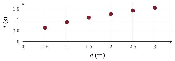
Original Photon diagram
(a) Explain why a model t=kd^{n} gives a straight line when \ln t is plotted against \ln d.
[2]
(b) Find the least-squares line of \ln t against \ln d, and hence find k and n.
[4]
(c) Sofia's teacher says n should be \frac{1}{2}. Comment on her result.
[2]
(d) Predict the time to roll 5 m and comment on the reliability of the prediction.
[3]
(e) Using n=\frac{1}{2}, find the value of k that minimises the sum of squared residuals of t against \sqrt{d}.
[5]
Show solutionHide solution
(a) t=kd^{n}\Rightarrow\ln t=\ln k+n\ln d [M1]; this has the form Y=c+nX with Y=\ln t and X=\ln d, a straight line of gradient n and intercept \ln k [R1].
(b) regression of \ln t on \ln d for the six readings [M1]; \ln t=-0.102+0.498\ln d [A1]; n=0.498 [A1]; k=e^{-0.102}=0.903 [A1].
(c) 0.498 is very close to 0.5 [R1]; the difference is well within what measurement error in six readings can produce, so the result is consistent with the teacher's value [R1].
(d) t=0.903\times5^{0.498} [M1] =2.01 s [A1]; 5 m lies outside the measured range 0.5 m to 3 m, so this is extrapolation, and the ramp may not even be that long [R1].
(e) S(k)=\sum\left(t-k\sqrt{d}\right)^{2} [M1]; \dfrac{dS}{dk}=-2\sum\sqrt{d}\left(t-k\sqrt{d}\right)=0 [M1]; k=\dfrac{\sum t\sqrt{d}}{\sum d} [A1]; \sum t\sqrt{d}=9.47 and \sum d=10.5 [A1]; k=0.902 [A1].

Final answer

  • (b) \ln t=-0.102+0.498\ln d, n=0.498, k=0.903
  • (c) n is close to 0.5, consistent
  • (d) 2.01 s, extrapolation beyond 3 m
  • (e) k=\frac{\sum t\sqrt d}{\sum d}=0.902.
Investigation 2

[16 marks]
This question asks you to model how a medicine leaves a patient's bloodstream.
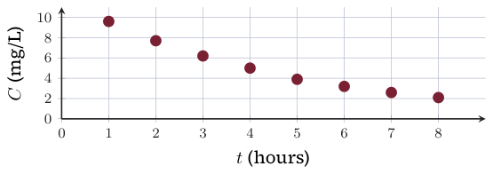
Fatima, a pharmacy student, measures the concentration C mg/L of a medicine in a patient's blood t hours after the dose has been absorbed.
\begin{array}{|l|r|c|r|c|r|c|r|c|}\hline t & 1 & 2 & 3 & 4 & 5 & 6 & 7 & 8\\\hline C & 9.6 & 7.7 & 6.2 & 5.0 & 3.9 & 3.2 & 2.6 & 2.1\\\hline\end{array}
Original Photon diagram
(a) Find the ratio of each concentration to the one before it. Explain why your ratios suggest an exponential model.
[3]
(b) Find the least-squares line of \ln C against t, and hence write down a model of the form C=Ae^{-kt}.
[4]
(c) Find the half-life of the medicine, that is the time for the concentration to halve.
[2]
(d) A second dose is due when the concentration falls to 1.0 mg/L. Find, according to the model, when this happens.
[2]
(e) The sum of squared residuals for the model, in C, is 0.0137. Explain what this value tells you.
[2]
(f) Fatima also fits the line C=9.76-1.05t. Find the time at which this line predicts C=0, and explain why this shows that it is unsuitable.
[3]
Show solutionHide solution
(a) \frac{7.7}{9.6}=0.802, \frac{6.2}{7.7}=0.805, 0.806, 0.780, 0.821, 0.812, 0.808 [M1]; all lie between 0.78 and 0.83 [A1]; a roughly constant ratio means the concentration is multiplied by the same factor each hour, which is exponential decay [R1].
(b) regression of \ln C on t [M1]; \ln C=2.48-0.218t [A1]; A=e^{2.475}=11.9 [A1]; k=0.218, so C=11.9e^{-0.218t} [A1].
(c) e^{-0.2179T}=\frac{1}{2} [M1]; T=\dfrac{\ln2}{0.2179}=3.18 hours [A1].
(d) 11.9e^{-0.2179t}=1 [M1]; t=\dfrac{\ln11.88}{0.2179}=11.4 hours [A1].
(e) the eight residuals are tiny, with a mean square of about 0.0017 [R1]; the model reproduces every reading to within about 0.1 mg/L, so it fits the data very well [R1].
(f) 9.76-1.05t=0 gives t=9.30 hours [A1]; after this the line gives a negative concentration [R1], which is impossible, whereas the concentration of a medicine only tends to zero [R1].

Final answer

  • (a) ratios about 0.80
  • (b) \ln C=2.48-0.218t, C=11.9e^{-0.218t}
  • (c) 3.18 hours
  • (d) 11.4 hours
  • (e) very small residuals
  • (f) 9.30 hours, then negative.

Investigation 3

[22 marks]
This question asks you to compare three models for the capacity of a rechargeable battery as it is used.
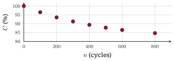
A laboratory measures the capacity C (% of new) of a battery after n charging cycles.
\begin{array}{|l|r|c|r|c|r|c|r|c|}\hline n & 0 & 100 & 200 & 300 & 400 & 500 & 600 & 800\\\hline C & 100 & 96.5 & 93.6 & 91.3 & 89.4 & 87.8 & 86.5 & 84.7\\\hline\end{array}
Original Photon diagram
(a) Find the linear model of best fit and its sum of squared residuals.
[3]
(b) Find an exponential model C=Ae^{-kn} by linearising, and its sum of squared residuals.
[4]
(c) A third model is C=80+20e^{-mn+c}. By plotting \ln\left(\frac{C-80}{20}\right) against n, find m and c, and the sum of squared residuals.
[5]
(d) Use each model to predict C after 1500 cycles.
[3]
(e) The manufacturer, Ms Tan, guarantees 70% capacity after 1500 cycles. Decide which models support her guarantee and which model you trust, giving reasons.
[4]
(f) Interpret the value 80 in the third model.
[1]
(g) Suggest an experiment that would help to decide between the models.
[2]
Show solutionHide solution
(a) regression of C on n [M1]; C=98.1-0.0190n [A1]; sum of squared residuals 10.5 [A1].
(b) regression of \ln C on n [M1]; \ln C=4.59-0.000207n [A1]; C=98.2e^{-0.000207n} [A1]; sum of squared residuals, in C, is 8.49 [A1].
(c) \ln\frac{C-80}{20}=0,\ -0.192,\ -0.386,\ \dots for the eight readings, all with C-80>0 [M1]; line y=-0.0162-0.00182n [A1]; m=0.00182 and c=-0.0162 [A1]; model values 80+20e^{-mn+c} [M1]; sum of squared residuals 0.169 [A1].
(d) linear 69.6 [A1]; exponential 72.0 [A1]; third model 81.3 [A1].
(e) the linear model gives 69.6%, below 70%, so only the exponential and third models support the guarantee [R1]; the third model has by far the smallest sum of squares, 0.169 against 10.5 and 8.49 [R1]; it levels off, which the first two cannot do, and a battery's capacity loss does slow down [R1]; all three predictions are extrapolations beyond 800 cycles [R1].
(f) the capacity (%) towards which the battery settles after a very large number of cycles [R1].
(g) test a battery to 1500 cycles or beyond [R1]; compare the measured capacities with each model's predictions, or repeat with several batteries [R1].

Final answer

  • (a) C=98.1-0.0190n, SSR 10.5
  • (b) C=98.2e^{-0.000207n}, SSR 8.49
  • (c) m=0.00182, c=-0.0162, SSR 0.169
  • (d) 69.6, 72.0, 81.3
  • (e) third model best
  • (f) long-term floor 80%.

Investigation 4

[20 marks]
This question asks you to decide between a power model and a quadratic model for the stopping distance of a car.
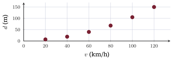
A road-safety team measures the total stopping distance d metres of a car braking from a speed of v km/h.
\begin{array}{|l|r|r|r|r|r|r|}\hline v & 20 & 40 & 60 & 80 & 100 & 120\\\hline d & 7 & 19 & 40 & 68 & 105 & 150\\\hline\end{array}
Original Photon diagram
(a) Find a power model d=kv^{n} by regression of \ln d on \ln v.
[4]
(b) Find the sum of squared residuals of the power model.
[3]
(c) Find the quadratic model of best fit and its coefficient of determination.
[3]
(d) Find the sum of squared residuals of the quadratic model.
[2]
(e) Use both models to predict the stopping distance at 150 km/h.
[2]
(f) Explain why physics suggests that a stopping distance contains a term in v and a term in v^{2}.
[3]
(g) A stopping distance should be zero at zero speed, but the quadratic model has a constant term of 2.90. Comment on this, and on the exponent in the power model.
[3]
Show solutionHide solution
(a) regression of \ln d on \ln v for the six readings [M1]; \ln d=-3.30+1.72\ln v [A1]; n=1.72 [A1]; k=e^{-3.30}=0.0369 [A1].
(b) model values 0.0369v^{1.72} at the six speeds [M1]; residuals d-\text{model} [M1]; sum of squares 124 [A1].
(c) quadratic regression of d on v [M1]; d=0.0102v^{2}-0.00125v+2.90 [A1]; R^{2}=1.00 (0.99998) [A1].
(d) model values and residuals [M1]; sum of squares 0.236 [A1].
(e) power model 205 m [A1]; quadratic model 233 m [A1].
(f) the driver travels at speed v during the reaction time, so the reaction distance is proportional to v [R1]; braking removes the kinetic energy \frac{1}{2}mv^{2} with a constant force, so the braking distance is proportional to v^{2} [R1]; the total distance is the sum, a quadratic in v [R1].
(g) the constant 2.90 m is small beside distances of up to 150 m and is probably measurement error, so the model is acceptable for speeds in the range [R1]; but it is not exactly zero at v=0, so the model should not be used at very low speeds [R1]; an exponent of 1.72 rather than 2 and a sum of squares of 124 against 0.236 show that the power model does not describe the mechanism [R1].

Final answer

  • (a) d=0.0369v^{1.72}
  • (b) 124
  • (c) d=0.0102v^2-0.00125v+2.90, R^2\approx1
  • (d) 0.236
  • (e) 205 m and 233 m.

Investigation 5

[20 marks]
This question asks you to decide whether growth is exponential or follows a power law.
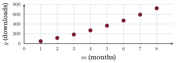
Hamid launches a podcast. The number of downloads y in month m after the launch is shown.
\begin{array}{|l|r|c|r|c|r|c|r|c|}\hline m & 1 & 2 & 3 & 4 & 5 & 6 & 7 & 8\\\hline y & 48 & 115 & 185 & 270 & 365 & 470 & 590 & 720\\\hline\end{array}
Original Photon diagram
(a) Find the least-squares line of \ln y against m, and hence an exponential model y=Ae^{km}. State the coefficient of determination of the line.
[3]
(b) Find the least-squares line of \ln y against \ln m, and hence a power model y=am^{n}. State the coefficient of determination of the line.
[3]
(c) Use your coefficients of determination to decide which model is better.
[2]
(d) Find the sum of squared residuals, in y, for each model.
[4]
(e) Explain why it is fair to compare the two coefficients of determination in (c).
[2]
(f) Predict the number of downloads in month 12 using each model.
[2]
(g) Using the power model, find the factor by which downloads are multiplied when the number of months doubles.
[2]
(h) Give one reason why the power model might still be unreliable for month 12.
[2]
Show solutionHide solution
(a) regression of \ln y on m [M1]; \ln y=3.94+0.360m and y=51.2e^{0.360m} [A1]; R^{2}=0.936 [A1].
(b) regression of \ln y on \ln m [M1]; \ln y=3.84+1.29\ln m and y=46.5m^{1.29} [A1]; R^{2}=0.999 (0.9987) [A1].
(c) the power model has the larger R^{2}, 0.999 against 0.936 [R1]; so the power model fits the data better [R1].
(d) model values for each model [M1]; residuals y-\text{model} in downloads [M1]; exponential 47 500 [A1]; power 1520 [A1].
(e) both lines have the same dependent variable, \ln y [R1]; so both R^{2} measure the share of the variation of \ln y that the line explains [R1].
(f) exponential 3850 [A1]; power 1160 [A1].
(g) 2^{n}=2^{1.29}=2.45 [M1], so downloads are multiplied by about 2.45 [A1].
(h) month 12 lies beyond the data, which stop at month 8 [R1]; the audience cannot grow for ever, or the podcast could lose listeners, so a smooth law may fail [R1].

Final answer

  • (a) y=51.2e^{0.360m}, R^2=0.936
  • (b) y=46.5m^{1.29}, R^2=0.999
  • (c) power
  • (d) 47 500 and 1520
  • (f) 3850 and 1160
  • (g) 2.45.

Investigation 6

[22 marks]
This question asks you to fit a logistic model with a known ceiling and to compare it with a quadratic model.
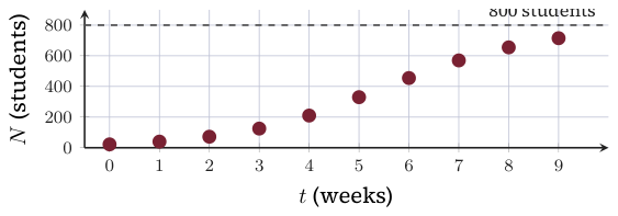
An app is launched in a school of 800 students. The number N of students using the app t weeks after the launch is shown.
\begin{array}{|l|r|c|r|c|r|c|r|c|r|c|}\hline t & 0 & 1 & 2 & 3 & 4 & 5 & 6 & 7 & 8 & 9\\\hline N & 22 & 40 & 72 & 125 & 210 & 330 & 455 & 570 & 655 & 715\\\hline\end{array}
Original Photon diagram
The company uses the model N=\dfrac{800}{1+ae^{-bt}}.
(a) Find \ln\left(\frac{800}{N}-1\right) for t=0 and for t=9.
[2]
(b) Find the least-squares line of \ln\left(\frac{800}{N}-1\right) against t, and hence find a and b.
[4]
(c) Use the model to predict N at t=6, and compare it with the reading.
[2]
(d) Find the time at which half of the students are using the app.
[2]
The rate of growth satisfies \dfrac{dN}{dt}=\dfrac{b}{800}N(800-N).
(e) Find the greatest rate of growth, and say when it occurs and what it means.
[4]
(f) Find the time at which 90% of the students are using the app.
[3]
(g) Give one reason why the ceiling 800 may be unrealistic.
[2]
A quadratic model N=4.81t^{2}+42.4t-8.56 is also fitted to the data.
(h) Find when the quadratic model predicts more than 800 students, and explain why this makes it unsuitable.
[3]
Show solutionHide solution
(a) t=0: \ln\left(\frac{800}{22}-1\right)=3.57 [A1]; t=9: \ln\left(\frac{800}{715}-1\right)=-2.13 [A1].
(b) transformed list for the ten readings [M1]; y=3.57-0.637t [A1]; b=0.637 [A1]; a=e^{3.574}=35.7 [A1].
(c) N(6)=\dfrac{800}{1+35.65e^{-0.637\times6}}=449 [A1]; the reading is 455, so the model is 6 students too low, a very close fit [R1].
(d) N=400 means ae^{-bt}=1 [M1]; t=\dfrac{\ln35.65}{0.637}=5.61 weeks [A1].
(e) the growth rate is greatest when N=400, half of 800 [M1]; \frac{b}{800}\times400\times400=\frac{800b}{4} [M1]; =127 students per week [A1]; it occurs about 5.6 weeks after launch, when 400 students are using the app [R1].
(f) N=720 gives \frac{800}{720}-1=\frac{1}{9}, so ae^{-bt}=\frac{1}{9} [M1]; t=\dfrac{\ln(9\times35.65)}{0.637} [M1]; =9.06 weeks [A1].
(g) not every student has a phone, or wants the app, so the number who will ever use it may be less than 800 [R1]; the ceiling was assumed, not found from the data [R1].
(h) 4.81t^{2}+42.4t-8.56=800 [M1]; t=9.29 weeks [A1]; after 9.3 weeks the model predicts more users than there are students, which is impossible, and it keeps growing, unlike the logistic model [R1].

Final answer

  • (a) 3.57 and −2.13
  • (b) a=35.7, b=0.637
  • (c) 449 against 455
  • (d) 5.61 weeks
  • (e) 127 students per week at 5.6 weeks
  • (f) 9.06 weeks
  • (h) 9.29 weeks.

Investigation 7

[26 marks]
This question asks you to decide which of two well-fitting models to trust for a long-range prediction.
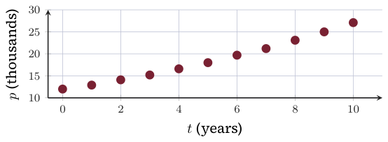
The population p (thousands) of a new town t years after it was founded is shown.
\begin{array}{|l|r|c|r|c|r|c|r|c|r|c|r|}\hline t & 0 & 1 & 2 & 3 & 4 & 5 & 6 & 7 & 8 & 9 & 10\\\hline p & 12.0 & 12.9 & 14.1 & 15.2 & 16.6 & 18.0 & 19.7 & 21.2 & 23.1 & 25.0 & 27.1\\\hline\end{array}
Original Photon diagram
(a) Find the linear model of best fit and its coefficient of determination.
[2]
(b) Describe the pattern of the residuals of the linear model and explain what it shows.
[3]
(c) Find the quadratic model of best fit and its sum of squared residuals.
[3]
(d) Find an exponential model p=Ae^{kt} by regression of \ln p on t, and its sum of squared residuals for p.
[4]
(e) Find the annual percentage growth rate and the doubling time given by the exponential model.
[3]
(f) Use the quadratic and exponential models to predict the population at t=20.
[2]
(g) The quadratic model has the smaller sum of squared residuals. Explain why a planner might still prefer the exponential model, and why she might prefer neither.
[5]
(h) The town has land for at most 60 000 people. Find when the exponential model reaches this limit, and suggest how the model should be changed.
[4]
Show solutionHide solution
(a) p=11.1+1.51t [A1]; R^{2}=0.988 [A1].
(b) residuals of the linear model, p-(11.1+1.51t), are positive at t=0 and t=10 and negative in the middle [R1]; they form a U-shaped pattern, not a random scatter [R1]; so the growth is curved (accelerating) and the straight line is not an appropriate model, in spite of R^{2}=0.988 [R1].
(c) quadratic regression of p on t [M1]; p=0.0601t^{2}+0.908t+12.0 [A1]; sum of squared residuals 0.0295 [A1].
(d) regression of \ln p on t [M1]; \ln p=2.48+0.0822t [A1]; p=11.9e^{0.0822t} [A1]; sum of squared residuals for p is 0.0444 [A1].
(e) growth factor per year e^{0.0822}=1.0857 [M1]; 8.56% per year [A1]; doubling time \dfrac{\ln2}{0.0822}=8.44 years [A1].
(f) quadratic 54.2 thousand [A1]; exponential 61.8 thousand [A1].
(g) the two sums of squares, 0.0295 and 0.0444, are both tiny, so the better fit is not decisive [R1]; the exponential model has parameters with a meaning, a constant percentage growth of 8.56% a year, which can be checked against a reason for growth [R1]; the quadratic coefficients have no such meaning [R1]; both models predict growth without limit, and they disagree by about 7.6 thousand people at t=20, well outside the data [R1]; real towns are limited by land and jobs, so a model with a ceiling may be better than either [R1].
(h) 11.9e^{0.0822t}=60 [M1]; t=\dfrac{\ln(60/11.9)}{0.0822}=19.6 years [A1]; the town cannot grow past its land, so growth must slow down [R1]; use a logistic model with L=60 [R1].

Final answer

  • (a) p=11.1+1.51t, R^2=0.988
  • (b) positive at the ends, negative in the middle
  • (c) p=0.0601t^2+0.908t+12.0, SSR 0.0295
  • (d) p=11.9e^{0.0822t}, SSR 0.0444
  • (e) 8.56%, 8.44 years
  • (f) 54.2 and 61.8 thousand
  • (h) 19.6 years; logistic with L=60.

Investigation 8

[26 marks]
This question asks you to choose the ceiling of a logistic model by comparing sums of squared residuals.
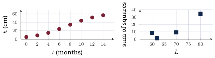
A biologist measures the height h cm of a mangrove sapling every two months, t months after planting.
\begin{array}{|l|r|c|r|c|r|c|r|c|}\hline t & 0 & 2 & 4 & 6 & 8 & 10 & 12 & 14\\\hline h & 5.1 & 9.0 & 15.0 & 24.1 & 34.5 & 44.0 & 51.5 & 56.8\\\hline\end{array}
She models the height by h=\dfrac{L}{1+ae^{-bt}}, where L, a and b are constants. For a chosen L, she fits the line \ln\left(\frac{L}{h}-1\right)=\ln a-bt by regression. The table gives the sum of squared residuals, in h, for four values of L.
\begin{array}{|l|r|r|r|r|}\hline L & 60 & 62 & 70 & 80\\\hline \text{sum of squares} & 8.25 & 1.17 & 9.24 & 34.5\\\hline\end{array}
Original Photon diagram
(a) Explain why L must be greater than 56.8.
[1]
(b) Take L=65. Find the least-squares line of \ln\left(\frac{65}{h}-1\right) against t, and hence find a and b.
[4]
(c) Find the sum of squared residuals for L=65.
[3]
(d) State which of L=60,62,65,70,80 fits best, and explain, using the sums of squares, why the best value of L must lie between 62 and 70.
[3]
The height satisfies \dfrac{dh}{dt}=\dfrac{b}{L}h(L-h).
(e) For L=65, find the time of fastest growth, the height then, and the greatest rate of growth.
[5]
(f) Find the time at which the height reaches 90% of L.
[2]
(g) A student tries L=63.5. Find the sum of squared residuals and comment on what it shows about the choice in (d).
[3]
(h) Explain why predictions for t>14 depend strongly on the value chosen for L.
[2]
(i) Use the model with L=65 to predict the height at t=30, and comment on its reliability.
[3]
Show solutionHide solution
(a) \ln\left(\frac{L}{h}-1\right) is undefined unless \frac{L}{h}>1 for every reading, so L must exceed the largest height, 56.8 [R1].
(b) \ln\left(\frac{65}{h}-1\right)=2.463,\ 1.828,\ 1.204,\ 0.529,\ -0.123,\ -0.740,\ -1.339,\ -1.935 [M1]; y=2.45-0.316t [A1]; b=0.316 [A1]; a=e^{2.449}=11.6 [A1].
(c) model values \dfrac{65}{1+11.6e^{-0.316t}} at the eight times [M1]; residuals h-\text{model} [M1]; sum of squares 0.914 [A1].
(d) L=65 [A1]; the sums of squares fall from 8.25 at 60 to 1.17 at 62 and 0.914 at 65, then rise to 9.24 at 70 [R1]; the sum of squares is larger at both 62 and 70 than at 65, so the smallest value occurs somewhere between 62 and 70, not necessarily at a tested value [R1].
(e) fastest growth when h=\frac{L}{2}=32.5 cm [M1]; ae^{-bt}=1 [M1]; t=\dfrac{\ln11.58}{0.316}=7.75 months [A1]; greatest rate \frac{b}{L}\times\frac{L}{2}\times\frac{L}{2}=\frac{bL}{4} [M1]; =5.14 cm per month [A1].
(f) h=58.5 gives \frac{65}{58.5}-1=\frac{1}{9}, so ae^{-bt}=\frac{1}{9} [M1]; t=\dfrac{\ln(9\times11.6)}{0.316}=14.7 months [A1].
(g) regression with L=63.5 [M1]; sum of squares 0.163 [A1]; this is far smaller than 0.914, so none of the five tested values was the best, and the sum of squares is very sensitive to L [R1].
(h) the readings stop at 14 months, before the curve has levelled off, so the data do not show the ceiling [R1]; values of L between 62 and 80 fit the readings tolerably and give long-term heights that differ by up to 18 cm [R1].
(i) \dfrac{65}{1+11.6e^{-0.316\times30}}=64.9 cm [A1]; this is almost exactly L, so the prediction is just the assumed ceiling [R1]; it is an extrapolation to more than twice the length of the data [R1].

Final answer

  • (a) L>56.8
  • (b) a=11.6, b=0.316
  • (c) 0.914
  • (d) L=65
  • (e) 7.75 months, 32.5 cm, 5.14 cm per month
  • (f) 14.7 months
  • (g) 0.163
  • (i) 64.9 cm.

Going further

Beyond the syllabus: the worked examples and investigations of the chapter's Going further pages.

Investigation

[25 marks]
Worked investigation 1: How tall does bamboo grow.
This question asks you to fit an exponential model and then a logistic model to the height of a bamboo shoot.
Mei measures the height h cm of a bamboo shoot every two days, where t is the time in days.
\begin{array}{|l|r|c|r|c|r|c|r|c|r|c|}\hline t & 0 & 2 & 4 & 6 & 8 & 10 & 12 & 14 & 16 & 18\\\hline h & 5 & 9 & 16 & 28 & 46 & 70 & 95 & 115 & 128 & 135\\\hline\end{array}
(a) For the first five readings only, find the least-squares line of \ln h against t, and hence write down a model of the form h=Ae^{kt}.
[3]
(b) Find the doubling time given by this model.
[2]
(c) Use this model to predict the height at t=18, and comment.
[2]
Mei now uses a logistic model h=\dfrac{L}{1+ae^{-bt}}, with L=140.
(d) Show that \ln\left(\dfrac{L}{h}-1\right)=\ln a-bt.
[3]
(e) Using all ten readings, find the least-squares line of \ln\left(\frac{140}{h}-1\right) against t, and hence find a and b.
[4]
(f) Use the logistic model to predict the height at t=10, and find the percentage error.
[2]
(g) Mei's friend suggests L=150, which gives a=28.794 and b=0.31812. The sum of squared residuals for L=140 is 64.8. Find the sum of squared residuals for L=150 and state which value of L fits better.
[4]
(h) For the model with L=150, find the time at which the shoot is growing fastest, and its height then.
[3]
(i) Explain why neither model should be used to predict the height after 60 days.
[2]
Show solutionHide solution
(a) \ln h for t=0,2,4,6,8: 1.609,\ 2.197,\ 2.773,\ 3.332,\ 3.829 [M1]
\ln h=1.633+0.2787\,t [A1]
h=e^{1.633}e^{0.2787t}=5.12\,e^{0.279t} [A1]
(b) e^{kT}=2, so T=\dfrac{\ln 2}{k} [M1]
T=\dfrac{\ln2}{0.2787}=2.49 days [A1]
(c) h(18)=5.12\,e^{0.2787\times18}=772 cm [A1]
the reading is 135 cm: the model overshoots by a factor of nearly six because the shoot's growth slows as it gets tall [R1]
(d) h=\dfrac{L}{1+ae^{-bt}}\ \Rightarrow\ \dfrac{L}{h}=1+ae^{-bt} [M1]
\dfrac{L}{h}-1=ae^{-bt} [A1]
\ln\left(\dfrac{L}{h}-1\right)=\ln a+\ln e^{-bt} [M1]
\ln\left(\dfrac{L}{h}-1\right)=\ln a-bt [AG]
(e) \ln\left(\frac{140}{h}-1\right) for the ten readings: 3.296,\ 2.678,\ \dots,\ -3.296 [M1]
y=3.48-0.362\,t [A1]
b=0.362 [A1]
a=e^{3.48111}=32.5 [A1]
(f) h(10)=\dfrac{140}{1+32.5\,e^{-0.362\times10}}=75.0 cm [A1]
\dfrac{|75.0-70|}{70}\times100=7.18\% [A1]
(g) model values \dfrac{150}{1+28.794e^{-0.31812t}} at t=0,2,\dots,18 [M1]
\sum(h-\text{model})^2 over the ten readings [M1]
25.2 [A1]
25.2<64.8, so L=150 fits better [R1]
(h) growth is fastest when h=\frac{L}{2}=75 cm [M1]
28.794e^{-0.31812t}=1 [M1]
t=\dfrac{\ln28.794}{0.31812}=10.6 days [A1]
(i) 60 days is far outside the data, which stop at 18 days: this is extrapolation [R1]
the exponential model gives about 9\times10^{7} cm; the logistic model's ceiling L was chosen by us, so the shoot may stop at another height or keep growing slowly [R1]

Final answer

  • (a) \ln h=1.633+0.2787t, h=5.12e^{0.279t}
  • (b) 2.49 days
  • (c) 772 cm
  • (e) a=32.5, b=0.362
  • (f) 75.0 cm, 7.18\%
  • (g) 25.2, so L=150
  • (h) 10.6 days, 75 cm.

Investigation

[24 marks]
Worked investigation 2: Power from a rooftop.
This question asks you to compare two models for the power produced by solar panels during a sunny day.
Arjun records the power output P kW of his rooftop panels each hour, where t is the time in hours after midnight.
\begin{array}{|l|r|c|r|c|r|c|r|c|r|c|r|c|r|}\hline t & 6 & 7 & 8 & 9 & 10 & 11 & 12 & 13 & 14 & 15 & 16 & 17 & 18\\\hline P & 0 & 1.1 & 2.0 & 2.8 & 3.5 & 3.8 & 4.0 & 3.9 & 3.4 & 2.9 & 2.1 & 1.0 & 0.1\\\hline\end{array}
(a) Find the quadratic model of best fit for P in terms of t, and its coefficient of determination.
[3]
(b) Arjun proposes P=4\sin\left(\dfrac{\pi(t-6)}{12}\right). Explain the values 4, 6 and 12 in context.
[3]
(c) Find the sum of squared residuals for each model.
[4]
(d) Use the trapezium rule with the 13 readings to estimate the energy, in kWh, produced between 06:00 and 18:00.
[3]
(e) Find the energy predicted by each model for 6\le t\le18.
[4]
(f) Find the times at which the quadratic model predicts zero output.
[2]
(g) State, with two reasons, which model you would use.
[3]
(h) Explain why neither model would describe a cloudy day.
[2]
Show solutionHide solution
(a) quadratic regression of P on t [M1]
P=-0.110\,t^{2}+2.64\,t-12.0 [A1]
R^{2}=0.995 [A1]
(b) 4 is the greatest output, 4 kW, reached at noon [R1]
6: the output is zero at t=6, so the Sun rises at 06:00 [R1]
12: the period is 24 h, so daylight lasts 12 h, to 18:00 [R1]
(c) residuals P-\text{model} at the 13 hours [M1]
quadratic: 0.112 [A1]
sine values 0,\ 1.035,\ 2.000,\ \dots,\ 4,\ \dots,\ 1.035,\ 0 [M1]
sine: 0.0421 [A1]
(d) \frac{1}{2}\left[0+0.1+2(1.1+\dots+1.0)\right], strip width 1 h [M1]
middle readings sum to 30.5 [A1]
\frac{1}{2}(0.1+61)=30.55\approx30.6 kWh [A1]
(e) \displaystyle\int_{6}^{18}(-0.110t^{2}+2.64t-11.98)\,dt [M1]
quadratic: 30.9 kWh [A1]
\displaystyle\int_{6}^{18}4\sin\frac{\pi(t-6)}{12}\,dt=\left[-\frac{48}{\pi}\cos\frac{\pi(t-6)}{12}\right]_{6}^{18} [M1]
\dfrac{48}{\pi}\left(1-(-1)\right)=\dfrac{96}{\pi}=30.6 kWh [A1]
(f) -0.110t^{2}+2.64t-12.0=0 [M1]
t=6.07 and t=17.97 [A1]
(g) the sine model [B1]
its sum of squares 0.0421 is less than 0.112, so its points lie closer to the data [R1]
it is zero at exactly 06:00 and 18:00 and symmetrical about noon; the quadratic is zero at 06:04 and 17:58 [R1]
(h) cloud cover makes the output rise and fall during the day [R1]
both models are smooth and symmetrical, so neither shows irregular dips [R1]

Final answer

  • (a) P=-0.110t^2+2.64t-12.0, R^2=0.995
  • (c) 0.112 and 0.0421
  • (d) 30.55 kWh
  • (e) 30.9 and \frac{96}{\pi}=30.6 kWh
  • (f) 6.07 and 17.97.

From the book

Photon Guidebook: Mathematics HL Paper 3 for the IB Diploma

Chapter 12 teaches fitting and comparing growth models: how the IB builds this kind of Paper 3 question, the techniques, marked worked investigations, and practice investigations like these.

About the book