Free worked solutions · 2026 Edition

IB Maths HL Paper 3 Chapter 9: Testing claims: the statistics suite worked solutions

Worked solutions to the investigations in Chapter 9 of Photon Guidebook: Mathematics HL Paper 3 for the IB Diploma (2026 Edition). Each solution shows every step with the mark it earns, the way an IB mark scheme does.

Chapter 9 of 18
10 practice questions
3 Going further
Free, no sign-up

Start with Investigations All 18 chapters

Investigations

The practice investigations of the chapter, each with its full worked solution and mark scheme.

Investigation 1

[16 marks]

This question asks you to compare noise levels in a library in an ordinary week and in an exam week.

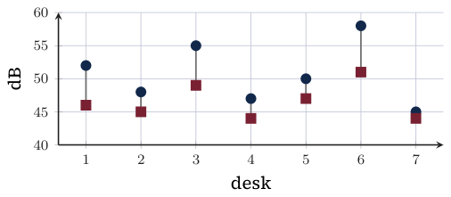
Nadia measures the sound level, in decibels (dB), at seven reading desks in her town library at the same time of day in an ordinary week and again in an exam week.

\begin{array}{|l|r|r|r|r|r|r|r|}\hline \text{Desk} & 1 & 2 & 3 & 4 & 5 & 6 & 7\\\hline \text{Ordinary week (dB)} & 52 & 48 & 55 & 47 & 50 & 58 & 45\\\hline \text{Exam week (dB)} & 46 & 45 & 49 & 44 & 47 & 51 & 44\\\hline\end{array}

(a) Name a suitable test to decide whether the mean sound level differs between the two weeks, and give a reason for your choice.

[2]

(b) Find the mean and standard deviation of the differences, ordinary minus exam.

[2]

(c) Carry out the test at the 5% significance level.

[5]

(d) State the assumption your test requires.

[1]

(e) Nadia's friend says the test shows that exam weeks cause the library to be quieter. Comment on this claim.

[2]

(f) Explain why measuring at the same time of day makes Nadia's comparison more valid.

[2]

(g) Suggest one further improvement to Nadia's data collection.

[2]

Show solutionHide solution

(a) paired t-test [R1]; the same seven desks are measured twice, so the two lists are not independent [R1].

(b) differences 6,3,6,3,3,7,1; \bar d=4.14 dB [A1]; s=2.19 dB [A1].

(c) \mathrm{H}_0\colon\mu_d=0, \mathrm{H}_1\colon\mu_d\ne0, where \mu_d is the mean difference in dB for all desks [A1]; paired t-test [M1]; t=5.00, p=0.00246 [A1 A1]; 0.00246<0.05: reject \mathrm{H}_0, the mean sound level differs between the weeks [R1].

(d) the differences are (approximately) normally distributed [R1].

(e) the test shows that the mean level differs, not why [R1]; for example, fewer visitors, or a different mix of users, in exam week [R1].

(f) the noise level varies through the day, so a time difference could produce a difference between weeks [R1]; measuring at the same time removes that source of variation, so the weeks are compared fairly [R1].

(g) for example, choose the desks at random and measure on several days [R1]; so the result does not depend on one day or one corner of the library [R1].

Final answer

(a) paired t-test, same desks measured twice
(b) \bar d=4.14 dB, s=2.19 dB
(c) t=5.00, p=0.00246<0.05, reject \mathrm{H}_0: the mean level differs
(d) differences normally distributed
(e) the test shows a difference, not its cause.

Investigation 2

[20 marks]

This question asks you to compare two ovens with a test based on ranks.

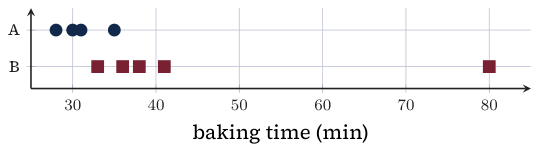
A bakery times how long, in minutes, a loaf takes to bake in each of two ovens. Oven A is used for 4 loaves and oven B for 5 loaves.

\begin{array}{|l|r|r|r|r|r|}\hline \text{Oven A (min)} & 31 & 28 & 35 & 30 & \\\hline \text{Oven B (min)} & 36 & 33 & 41 & 38 & 80\\\hline\end{array}

(a) Explain why a t-test may not be suitable for these data.

[2]

(b) Carry out a pooled two-sample t-test at the 5% level to test whether loaves bake faster in oven A, and state your conclusion.

[4]

In a rank-sum test, all 9 times are ranked together from shortest (rank 1) to longest (rank 9), and W is the sum of the ranks of the oven A times. If both ovens are equally fast, every set of 4 ranks from 1 to 9 is equally likely to belong to oven A.

(c) Show that W=11.

[2]

(d) Write down the smallest and largest possible values of W.

[2]

(e) Find the number of ways of choosing 4 ranks from 1 to 9, and list the sets of ranks that give W\le11.

[4]

(f) Hence find \mathrm{P}(W\le11) if both ovens are equally fast.

[2]

(g) At the 5% level, \mathrm{H}_0 is rejected when W\le12. State the conclusion of the rank-sum test, and explain why it differs from the conclusion in (b).

[4]

Show solutionHide solution

(a) one time, 80 minutes, is far from the others, so the data are not close to normal [R1]; with only 4 and 5 loaves the outlier has a large effect on the mean and the spread [R1].

(b) \mathrm{H}_0\colon\mu_A=\mu_B, \mathrm{H}_1\colon\mu_A<\mu_B [A1]; pooled two-sample t-test [M1]; t=-1.47, p=0.0928 [A1]; 0.0928>0.05: do not reject \mathrm{H}_0, no evidence at the 5% level that oven A is faster [R1].

(c) ranked times 28,30,31,33,35,36,38,41,80 have ranks 1 to 9 [M1]; oven A has ranks 3,1,5,2, so W=11 [A1].

(d) smallest 1+2+3+4=10 [A1]; largest 6+7+8+9=30 [A1].

(e) \binom94=126 sets [A1]; check the sets with sum at most 11 [M1]: \{1,2,3,4\} [A1] and \{1,2,3,5\} [A1].

(f) \mathrm{P}(W\le11)=\frac{2}{126} [M1] =0.0159 [A1].

(g) 11\le12, so reject \mathrm{H}_0: evidence that oven A is faster [A1 R1]; the outlier 80 inflates oven B's mean and spread, which weakens the t-test [R1], but in the rank-sum test it is only the largest rank, 9, however large it is [R1].

Final answer

(b) t=-1.47, p=0.0928>0.05, do not reject
(c) ranks 3,1,5,2
(d) 10 and 30
(e) 126; \{1,2,3,4\} and \{1,2,3,5\}
(f) \frac{2}{126}=0.0159
(g) reject \mathrm{H}_0: oven A is faster; the outlier weakens the t-test but counts only as a rank.

Investigation 3

[24 marks]

This question asks you to model bus arrivals at a stop and to test whether a new timetable has increased them.

Ibrahim counts the number of buses that arrive at a stop in each of 100 five-minute intervals.

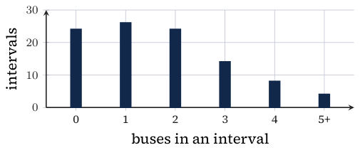
\begin{array}{|l|r|r|r|r|r|r|}\hline \text{Buses} & 0 & 1 & 2 & 3 & 4 & \text{5 or more}\\\hline \text{Intervals} & 24 & 26 & 24 & 14 & 8 & 4\\\hline\end{array}

He models the number of buses in a five-minute interval by a Poisson distribution with mean 1.7.

(a) Find the expected number of intervals for each number of buses.

[3]

(b) Test, at the 5% level, whether the Poisson model with mean 1.7 fits the data. Explain how you chose the degrees of freedom.

[6]

(c) Suggest one reason why bus arrivals might not follow a Poisson distribution.

[1]

After a new timetable, Ibrahim will count the buses in one hour, Y, to test whether the mean rate has increased.

(d) Write down the distribution of Y if the rate is unchanged.

[1]

(e) Find the critical region for a test at the 5% level.

[3]

(f) Given that the new mean rate is in fact 2.5 buses per five minutes, find the probability that the test fails to detect the increase.

[3]

(g) Ibrahim counts 27 buses in the hour. State his conclusion.

[2]

(h) Explain what a Type II error would mean for Ibrahim in this context.

[2]

(i) Ibrahim's friend suggests counting during the morning rush hour only. Comment on this suggestion.

[3]

Show solutionHide solution

(a) 100\times\mathrm{P}(X=x) with X\sim\mathrm{Po}(1.7) [M1]; 18.3,\ 31.1,\ 26.4,\ 15.0,\ 6.36 [A1]; the last cell is 100\times\mathrm{P}(X\ge5)=2.96 [A1].

(b) \mathrm{H}_0: the number of buses follows \mathrm{Po}(1.7); \mathrm{H}_1: it does not [A1]; the expected count 2.96 is below 5, so merge “5 or more” with 4 (observed 12, expected 9.32) [M1]; 5 cells, and the mean 1.7 is given so no parameter is estimated: \mathrm{df}=5-1=4 [M1]; \chi^2=3.67 [A1]; p=0.452 [A1]; 0.452>0.05: do not reject \mathrm{H}_0, the model is consistent with the data [R1].

(c) for example, buses are timetabled, so arrivals are not independent and tend to bunch [R1].

(d) Y\sim\mathrm{Po}(20.4) [A1].

(e) \mathrm{H}_1: the rate has increased, so find the smallest c with \mathrm{P}(Y\ge c)\le0.05 [M1]; \mathrm{P}(Y\ge28)>0.05 and \mathrm{P}(Y\ge29)=0.0422 [M1]; critical region Y\ge29 [A1].

(f) if the rate is 2.5 per five minutes, Y\sim\mathrm{Po}(30) [M1]; the test fails to detect it when Y\le28 [M1]; \mathrm{P}(Y\le28)=0.403 [A1].

(g) 27 is not in the critical region [R1]; do not reject \mathrm{H}_0: no evidence that the mean rate has increased [R1].

(h) concluding that there is no evidence of an increase [R1] when the mean number of buses has in fact increased [R1].

(i) the rush hour has a higher rate than an ordinary hour [R1]; so a count in the rush hour would be compared with the wrong baseline and could look like an increase when none has happened [R1]; Ibrahim should compare the same hour of the day before and after the change [R1].

Final answer

(a) 18.3,31.1,26.4,15.0,6.36,2.96
(b) merge 4 with 5 or more, \mathrm{df}=5-1=4 (mean given), \chi^2=3.67, p=0.452, do not reject
(d) \mathrm{Po}(20.4)
(e) Y\ge29
(f) 0.403
(g) 27 not in region, no evidence of an increase.

Investigation 4

[27 marks]

This question asks you to investigate whether screen time before bed is linked to sleep, and how much the evidence can show.

A school has 360 students in Grade 11 and 240 in Grade 12. Lena wants a sample of 60 students for a survey about screen use before bed.

(a) Find the number of students from each grade in a stratified sample of 60, and give one advantage of stratified sampling here.

[3]

Lena records each student's usual screen time in the hour before bed and how rested they feel in the morning.

\begin{array}{|l|r|r|r|}\hline & \text{Rested} & \text{Neutral} & \text{Tired}\\\hline \text{Under 20 minutes} & 12 & 6 & 4\\\hline \text{20 to 40 minutes} & 8 & 7 & 7\\\hline \text{Over 40 minutes} & 3 & 5 & 8\\\hline\end{array}

(b) Test, at the 5% significance level, whether feeling rested is independent of screen time.

[6]

(c) Lena's teacher is concerned about one of the expected frequencies. Identify it, explain the concern, and suggest how the table could be changed.

[3]

Lena also records, for eight students, the minutes of screen time before bed and the minutes taken to fall asleep.

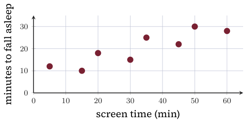
\begin{array}{|l|r|r|r|r|r|r|r|r|}\hline \text{Screen time (min)} & 5 & 15 & 20 & 30 & 35 & 45 & 50 & 60\\\hline \text{Time to fall asleep (min)} & 12 & 10 & 18 & 15 & 25 & 22 & 30 & 28\\\hline\end{array}

(d) Rank both variables and find the value of Spearman's coefficient r_s for Lena's eight students.

[3]

(e) For 8 pairs, the critical value of r_s for a one-tailed test at the 5% level is 0.643. Test whether there is a positive association.

[3]

(f) Explain why Spearman's coefficient might be preferred to Pearson's coefficient here.

[2]

(g) Lena concludes that screens before bed cause students to take longer to fall asleep. Comment on her conclusion.

[2]

(h) Lena carries out three independent tests, each at the 5% level, when every null hypothesis is true. Find the probability that at least one of them leads to a Type I error.

[3]

(i) Suggest how Lena could design a study that tests her claim about cause more convincingly.

[2]

Show solutionHide solution

(a) 60\times\frac{360}{600}=36 [M1] from Grade 11 and 60\times\frac{240}{600}=24 from Grade 12 [A1]; every grade is represented in proportion to its size, so neither grade is missed by chance [R1].

(b) \mathrm{H}_0: feeling rested is independent of screen time; \mathrm{H}_1: it is not [A1]; \chi^2 test for independence, with expected counts from row total times column total over 60 [M1]; \chi^2=6.18 [A1]; \mathrm{df}=(3-1)(3-1)=4 [A1]; p=0.186 [A1]; 0.186>0.05: do not reject \mathrm{H}_0, no evidence at the 5% level that feeling rested depends on screen time [R1].

(c) the expected count for over 40 minutes and neutral is \frac{16\times18}{60}=4.8 [A1]; it is below 5, so the \chi^2 approximation is unreliable [R1]; merge two columns (for example neutral with tired) or two rows [A1].

(d) ranks of screen time 1 to 8 in order, and of time to fall asleep 2,1,4,3,6,5,8,7 [M1]; \sum d^2=8 [A1]; r_s=1-\frac{6\times8}{8\times63}=0.905 [A1].

(e) \mathrm{H}_0: no association, \mathrm{H}_1: positive association [A1]; 0.905>0.643 [M1]; reject \mathrm{H}_0: evidence of a positive association between screen time and time to fall asleep [R1].

(f) Spearman's coefficient measures any increasing relationship, not only a straight line [R1]; it uses ranks, so one extreme value has less effect [R1].

(g) correlation does not show cause [R1]; a hidden factor, such as worry or a late-night routine, could raise both screen time and time to fall asleep [R1].

(h) 1-0.95^3 [M1] =0.143 [A1]; repeating tests makes at least one false positive more likely than 5% [R1].

(i) give some students a screen-free hour before bed and others not, deciding who is in which group at random [R1]; measure time to fall asleep for both groups over several nights, so the groups differ only in screen use [R1].

Final answer

(a) 36 and 24
(b) \chi^2=6.18, \mathrm{df}=4, p=0.186, do not reject
(c) expected 4.8 (over 40 minutes, neutral) is below 5; merge two columns or rows
(d) r_s=0.905
(e) 0.905>0.643, reject, positive association
(h) 1-0.95^3=0.143.

Investigation 5

[16 marks]

This question asks you to test whether bags of rice are filled below their label mass.

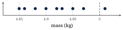
Efua runs a grocery stall. The bags of rice she buys are labelled 5 kg. She weighs 9 bags, and their masses, in kg, are

\begin{array}{|l|r|r|r|r|c|r|r|r|r|}\hline \text{Bag} & 1 & 2 & 3 & 4 & 5 & 6 & 7 & 8 & 9\\\hline \text{Mass (kg)} & 4.92 & 4.88 & 5.01 & 4.85 & 4.95 & 4.90 & 4.97 & 4.86 & 4.93\\\hline\end{array}

(a) Efua suspects that the mean mass of all such bags is less than 5 kg. State suitable hypotheses.

[2]

(b) Find the mean and the standard deviation of the nine masses.

[2]

(c) Carry out a test of Efua's suspicion at the 5% significance level.

[5]

(d) Find a 95% confidence interval for the mean mass of all such bags.

[3]

(e) State one assumption needed for the test in (c).

[1]

(f) Explain why the interval in (d) agrees with your conclusion in (c).

[2]

(g) All nine bags came from the top layer of one pallet. Explain why this may affect Efua's conclusion.

[1]

Show solutionHide solution

(a) \mathrm{H}_0\colon\mu=5 [A1]; \mathrm{H}_1\colon\mu<5, where \mu is the mean mass, in kg, of all such bags [A1].

(b) \bar x=4.92 kg [A1]; s=0.0525 kg [A1].

(c) one-sample t-test [M1]; t=-4.63 [A1]; p=0.000843 [A1]; 0.000843<0.05 [A1]: reject \mathrm{H}_0, there is evidence that the mean mass is less than 5 kg [R1].

(d) 4.919\pm t_8(0.975)\times\frac{0.0525}{\sqrt9} [M1]; (4.88,\,4.96) kg [A1]; we are 95% confident that the mean mass of all such bags is between 4.88 kg and 4.96 kg [R1].

(e) the masses are (approximately) normally distributed [R1].

(f) the label mass, 5 kg, lies outside the interval [R1]; the whole interval is below 5 kg, which agrees with the evidence of a lower mean [R1].

(g) bags from one place on one pallet may not represent all bags, for example if bags settle during transport [R1].

Final answer

(a) \mathrm{H}_0\colon\mu=5, \mathrm{H}_1\colon\mu<5
(b) \bar x=4.92 kg, s=0.0525 kg
(c) t=-4.63, p=0.000843<0.05, reject
(d) (4.88,4.96) kg
(e) masses normally distributed
(f) 5 lies outside the interval.

Investigation 6

[20 marks]

This question asks you to test whether visits to a museum are equally likely on each weekday, and then to question a second test.

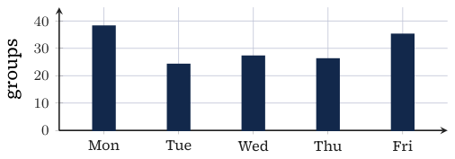
Elif counts the school groups that arrive at a museum on each weekday of one week, 150 groups in all.

\begin{array}{|l|r|r|r|r|r|}\hline \text{Day} & \text{Mon} & \text{Tue} & \text{Wed} & \text{Thu} & \text{Fri}\\\hline \text{Groups} & 38 & 24 & 27 & 26 & 35\\\hline\end{array}

(a) Elif wishes to test whether groups are equally likely to arrive on each weekday. State the hypotheses and find the expected number of groups for each day.

[2]

(b) Write down the number of degrees of freedom, and explain why no parameter has been estimated.

[2]

(c) Carry out the test, using a significance level of 5%.

[4]

(d) Write down the critical value for the test at the 5% level, and explain how it agrees with your conclusion in (c).

[2]

The museum manager notices that Monday and Friday together account for 73 of the 150 groups. She tests, at the 5% level, whether the probability that a group arrives on Monday or Friday is greater than \frac25.

(e) Carry out the manager's test, using a binomial distribution.

[4]

(f) Explain why the conclusion in (e) is less trustworthy than the conclusion in (c).

[2]

(g) State which day contributes most to the value of \chi^2 in (c), and give the contribution.

[2]

(h) Give one reason, in context, why one week of data may not show the usual pattern.

[2]

Show solutionHide solution

(a) \mathrm{H}_0: groups are equally likely on each weekday; \mathrm{H}_1: they are not [A1]; expected \frac{150}{5}=30 for each day [A1].

(b) 5 cells, so \mathrm{df}=5-1=4 [A1]; the expected counts come from the hypothesis (equal probabilities), not from the data, so nothing is estimated [R1].

(c) \chi^2 goodness of fit test with expected counts 30 [M1]; \chi^2=5.00 [A1]; p=0.287 [A1]; 0.287>0.05: do not reject \mathrm{H}_0, no evidence that arrivals are unequal across weekdays [R1].

(d) critical value 9.49 [A1]; 5.00<9.49, so \mathrm{H}_0 is not rejected, as in (c) [R1].

(e) \mathrm{H}_0\colon p=0.4, \mathrm{H}_1\colon p>0.4 [A1]; under \mathrm{H}_0, X\sim\mathrm{B}(150,0.4) [M1]; \mathrm{P}(X\ge73)=0.0193 [A1]; 0.0193<0.05: reject \mathrm{H}_0, evidence that Monday and Friday are busier than the other days [R1].

(f) the manager chose Monday and Friday after seeing which days were highest [R1]; a test chosen after looking at the data, among many possible tests, makes a chance result look significant [R1].

(g) Monday [R1]; its contribution is \frac{(38-30)^2}{30}=2.13 [A1].

(h) for example, a school holiday or an exhibition on one weekday, so that the week is not typical [R1 R1].

Final answer

(a) expected 30 each day
(b) \mathrm{df}=4, nothing estimated
(c) \chi^2=5.00, p=0.287, do not reject
(d) 9.49
(e) \mathrm{P}(X\ge73)=0.0193, reject
(f) the test was chosen after seeing the data
(g) Monday, 2.13.

Investigation 7

[20 marks]

This question asks you to build a two-tailed test for a proportion and to find how well it detects a change.

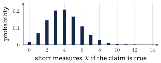
A drinks machine is claimed to dispense a short measure in 10% of cups. Ravi checks 40 cups and counts X, the number of short measures.

(a) State suitable hypotheses for a test of the claim, defining p.

[2]

Ravi will use a two-tailed test at the 5% level, with a critical region that has probability at most 0.025 in each tail.

(b) Find the critical region in the lower tail.

[2]

(c) Find the critical region in the upper tail.

[3]

(d) Write down the whole critical region and the actual significance level of the test.

[2]

(e) Ravi finds 8 short measures. State his conclusion.

[2]

(f) The machine in fact gives a short measure with probability 0.2. Find the probability that Ravi's test fails to detect this.

[3]

(g) Explain why a two-tailed test is appropriate here.

[2]

(h) Suggest how Ravi could reduce the probability in (f), and state one cost.

[2]

(i) Explain why the actual significance level in (d) is less than 5%.

[2]

Show solutionHide solution

(a) \mathrm{H}_0\colon p=0.1 [A1]; \mathrm{H}_1\colon p\ne0.1, where p is the probability that a cup is a short measure [A1].

(b) under \mathrm{H}_0, X\sim\mathrm{B}(40,0.1); \mathrm{P}(X\le0)=0.0148\le0.025 and \mathrm{P}(X\le1)=0.0805>0.025 [M1]; the lower region is X=0 [A1].

(c) find the smallest d with \mathrm{P}(X\ge d)\le0.025 [M1]; \mathrm{P}(X\ge8)=0.0419>0.025 and \mathrm{P}(X\ge9)=0.0155\le0.025 [M1]; the upper region is X\ge9 [A1].

(d) critical region X=0 or X\ge9 [A1]; actual significance level 0.0148+0.0155=0.0303 [A1].

(e) 8 is not in the critical region [R1]; do not reject \mathrm{H}_0: not enough evidence that the proportion of short measures differs from 10% [R1].

(f) if p=0.2, X\sim\mathrm{B}(40,0.2) [M1]; the test fails to detect this when 1\le X\le8 [M1]; probability =0.593 [A1].

(g) the claim of 10% could be wrong in either direction, and Ravi has no reason to expect one direction before sampling [R1 R1].

(h) check more cups [R1]; it takes more time and more drinks to be checked (or any sensible cost) [R1].

(i) the binomial distribution is discrete, so the probabilities of the tails jump in steps [R1]; no region has probability exactly 0.05, and the region is chosen so that each tail stays at most 0.025 [R1].

Final answer

(a) \mathrm{H}_0\colon p=0.1, \mathrm{H}_1\colon p\ne0.1
(b) X=0
(c) X\ge9
(d) X=0 or X\ge9, level 0.0303
(e) 8 not in the region, do not reject
(f) 0.593.

Investigation 8

[26 marks]

This question asks you to use a statistic defined in the question to test whether counts are more variable than a Poisson model allows.

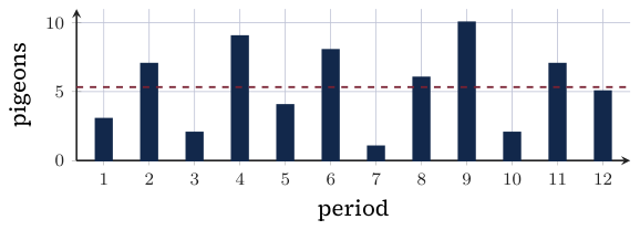
Sofia counts the pigeons that land at a feeder in each of 12 ten-minute periods.

\begin{array}{|l|r|r|r|r|c|r|r|r|r|c|r|r|}\hline \text{Period} & 1 & 2 & 3 & 4 & 5 & 6 & 7 & 8 & 9 & 10 & 11 & 12\\\hline \text{Pigeons} & 3 & 7 & 2 & 9 & 4 & 8 & 1 & 6 & 10 & 2 & 7 & 5\\\hline\end{array}

(a) Show that the mean number of pigeons per period is 5.33 to 3 significant figures, and find the sample variance.

[2]

(b) State how the variance of a Poisson distribution is related to its mean.

[1]

Sofia uses the statistic D=\dfrac{(n-1)s^2}{\bar x}, where n is the number of periods, \bar x the sample mean and s^2 the sample variance. If the counts follow a Poisson distribution, D is approximately \chi^2 with n-1 degrees of freedom. Larger values of D indicate more variability than a Poisson distribution allows.

(c) Calculate D for Sofia's data.

[2]

(d) State suitable hypotheses for a test of whether the counts are more variable than a Poisson distribution allows.

[1]

(e) Find the critical value at the 5% level and state the conclusion of the test.

[4]

(f) Calculate the p-value of Sofia's test.

[2]

(g) Explain why only large values of D lead to rejection of \mathrm{H}_0.

[2]

(h) Comment on the result, referring to the sample variance and the number of periods.

[2]

Suppose that Sofia had observed the same mean and the same sample variance in 24 periods.

(i) Find D and the new critical value, and state the conclusion.

[4]

(j) Explain, in context, what a Type II error would mean for Sofia.

[2]

(k) Suggest a reason, in context, why the counts might be more variable than a Poisson distribution.

[2]

(l) Suggest one change to the way Sofia collects her counts.

[2]

Show solutionHide solution

(a) sum 64, so \bar x=\frac{64}{12}=5.33 [A1]; sample variance s^2=8.79 [A1].

(b) the variance equals the mean [R1].

(c) D=\frac{11\times8.7879}{5.3333} [M1] =18.1 [A1].

(d) \mathrm{H}_0: the counts follow a Poisson distribution; \mathrm{H}_1: the counts are more variable than a Poisson distribution [A1].

(e) \mathrm{df}=12-1=11 [A1]; critical value 19.7 [A1]; 18.1<19.7 [M1]; do not reject \mathrm{H}_0: no evidence at the 5% level that the counts are more variable than Poisson [R1].

(f) p=0.0787 [A1]; 0.0787>0.05, so \mathrm{H}_0 is not rejected, as in (e) [R1].

(g) the alternative is greater variability, which makes D large [R1]; a small D would suggest less variability than Poisson, which is not the alternative being tested [R1].

(h) the sample variance is about 65% larger than the mean, which is a noticeable excess [R1]; with only 12 periods the test has little power, so the evidence is not strong enough to reject [R1].

(i) D=\frac{23\times8.7879}{5.3333}=37.9 [M1 A1]; critical value for \mathrm{df}=23 is 35.2 [A1]; 37.9>35.2: reject \mathrm{H}_0 [R1].

(j) concluding that there is no evidence of extra variability [R1] when the counts are in fact more variable than Poisson [R1].

(k) for example, pigeons arrive in flocks, so several land together and counts are not independent [R1 R1].

(l) for example, count for more periods, at different times of day [R1]; so that the test is more powerful and the pattern does not come from one time of day [R1].

Final answer

(a) \bar x=5.33, s^2=8.79
(b) variance equals mean
(c) D=18.1
(e) \mathrm{df}=11, critical value 19.7, do not reject
(f) p=0.0787
(i) D=37.9, critical value 35.2, reject.

Investigation 9

[16 marks]

This question asks you to compare a sign test with a paired t-test on the same data.

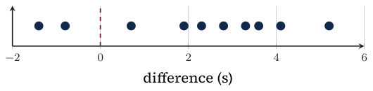
Ten club runners are timed over 400 m before and after a three-week training plan. The differences in time, before minus after, in seconds, are

\begin{array}{|l|r|r|r|r|c|r|r|r|r|r|}\hline \text{Runner} & 1 & 2 & 3 & 4 & 5 & 6 & 7 & 8 & 9 & 10\\\hline \text{Difference (s)} & 4.1 & 2.3 & -0.8 & 3.6 & 1.9 & 5.2 & -1.4 & 2.8 & 3.3 & 0.7\\\hline\end{array}

(a) Find the mean and the standard deviation of the differences.

[2]

(b) Use a paired t-test, with a 5% level of significance, to decide whether the plan reduces the mean time.

[5]

(c) A sign test counts the runners whose time fell. If the plan has no effect, each runner is equally likely to improve or not, independently. Carry out a sign test at the 5% level to test whether the plan helps.

[4]

(d) Explain why the conclusions of the two tests differ.

[2]

(e) Find the critical region for the sign test at the 5% level.

[2]

(f) State one assumption of the test in (b).

[1]

Show solutionHide solution

(a) \bar d=2.17 s [A1]; s=2.12 s [A1].

(b) \mathrm{H}_0\colon\mu_d=0, \mathrm{H}_1\colon\mu_d>0, where \mu_d is the mean reduction in time for all runners [A1]; paired t-test [M1]; t=3.24, p=0.00510 [A1 A1]; 0.00510<0.05: reject \mathrm{H}_0, evidence that the plan reduces the mean time [R1].

(c) 8 of the 10 runners improved; under \mathrm{H}_0, X\sim\mathrm{B}(10,0.5) [M1]; \mathrm{P}(X\ge8)=0.0547 [A1]; 0.0547>0.05 [R1]: do not reject \mathrm{H}_0, not enough evidence at the 5% level that the plan helps [R1].

(d) the sign test uses only whether each difference is positive, not how large it is [R1]; the large improvements of several runners are ignored, so it has less power to detect the improvement [R1].

(e) \mathrm{P}(X\ge9)=0.0107\le0.05 and \mathrm{P}(X\ge8)=0.0547>0.05 [M1]; critical region X\ge9 [A1].

(f) the differences are (approximately) normally distributed [R1].

Final answer

(a) \bar d=2.17 s, s=2.12 s
(b) t=3.24, p=0.00510, reject \mathrm{H}_0
(c) \mathrm{P}(X\ge8)=0.0547>0.05, do not reject
(d) the sign test ignores the sizes of the differences
(e) X\ge9
(f) differences normally distributed.

Investigation 10

[20 marks]

This question asks you to rebuild a table from percentages and to test whether satisfaction depends on how people travel.

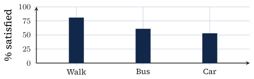
A transport survey asks 300 commuters how they travel and whether they are satisfied with their trip. Of the 300 commuters, 30% walk, 45% take the bus and 25% travel by car. Of the walkers, 80% are satisfied; of the bus users, 60%; of the car users, 52%.

(a) Construct the table of observed frequencies, with rows walk, bus and car and columns satisfied and not satisfied.

[3]

(b) Test, at the 1% significance level, whether satisfaction is independent of the way of travelling.

[5]

(c) Find the smallest expected frequency and state whether it makes the test unreliable.

[2]

(d) Write down the critical value for the test, and explain how it agrees with your conclusion in (b).

[2]

(e) State which way of travelling contributes most to the value of \chi^2, and give the contribution.

[2]

The measure V=\sqrt{\dfrac{\chi^2}{N}} is described as negligible if V<0.15, moderate if 0.15\le V<0.30 and strong if V\ge0.30, where N is the number of commuters.

(f) Calculate V and describe the strength of the association.

[3]

(g) All 300 commuters were surveyed at a bus station. Explain why this affects the conclusion.

[2]

(h) Explain how stratified sampling could improve the survey.

[1]

Show solutionHide solution

(a) walkers 0.30\times300=90, bus users 0.45\times300=135, car users 0.25\times300=75 [M1]; satisfied 0.8\times90=72, 0.6\times135=81, 0.52\times75=39 [A1]; not satisfied 18, 54, 36 [A1].

(b) \mathrm{H}_0: satisfaction is independent of the way of travelling; \mathrm{H}_1: it is not [A1]; \chi^2 test for independence [M1]; \chi^2=15.6 [A1]; \mathrm{df}=(3-1)(2-1)=2 [A1]; p=0.000405<0.01: reject \mathrm{H}_0, satisfaction depends on how people travel [R1].

(c) the smallest expected frequency is \frac{75\times108}{300}=27.0, for car users who are not satisfied [A1]; it is above 5, so the test is reliable [R1].

(d) critical value 9.21 [A1]; 15.6>9.21, so \mathrm{H}_0 is rejected, as in (b) [R1].

(e) walking [R1]; contribution 10.0 [A1].

(f) V=\sqrt{15.625/300} [M1] =0.228 [A1]; 0.15\le V<0.30: a moderate association [R1].

(g) everyone surveyed was at a bus station, so walkers and car users are under-represented and bus users over-represented, and bus users may differ from the others in satisfaction [R1 R1].

(h) sample a set number from each way of travelling, in proportion to its size, so that every group is represented [R1].

Final answer

(a) walk 72,18; bus 81,54; car 39,36
(b) \chi^2=15.6, \mathrm{df}=2, p=0.000405, reject \mathrm{H}_0
(c) 27.0, test reliable
(d) 9.21
(e) walking, 10.0
(f) V=0.228, moderate.

Going further

Beyond the syllabus: the worked examples and investigations of the chapter's Going further pages.

Investigation

[26 marks]

Worked investigation 1: Screen breaks at a call centre.

This question asks you to judge whether short screen-free breaks improve the reaction times of call-centre staff.

Priya manages a call centre. She measures the reaction time, in milliseconds (ms), of eight members of staff on a computer task, gives each of them a ten-minute screen-free break, and measures them again.

\begin{array}{|l|r|r|r|r|r|r|r|r|}\hline \text{Staff member} & A & B & C & D & E & F & G & H\\\hline \text{Before (ms)} & 312 & 298 & 335 & 290 & 305 & 321 & 287 & 342\\\hline \text{After (ms)} & 301 & 296 & 318 & 285 & 299 & 309 & 290 & 326\\\hline\end{array}

(a) Explain why Priya should analyse the differences, before minus after, rather than the two columns separately.

[1]

(b) Find the mean and the standard deviation of the differences.

[2]

(c) Test, at the 5% significance level, whether the break reduces the mean reaction time. State your hypotheses, the p-value and your conclusion.

[5]

(d) State one assumption that your test in (c) requires.

[1]

On another day, eight different members of staff are measured twice, one hour apart, with no break. Their differences, first minus second, in ms, are -2, 4, 1, -5, 3, 0, 6, -1.

(e) Carry out a pooled two-sample t-test at the 5% level to decide whether the mean improvement with a break is greater than the mean improvement without one.

[5]

(f) Explain why the test in (e) gives better evidence about the effect of the break than the test in (c).

[2]

A sign test counts how many of the eight differences in the table are positive. If the break has no effect, each difference is equally likely to be positive or negative, independently.

(g) Use a sign test at the 5% level to test whether the break reduces reaction times.

[3]

(h) Find a 95% confidence interval for the mean reduction in reaction time after a break, and interpret it.

[3]

(i) Explain, in context, what a Type I error would be in (c), and write down its probability.

[2]

(j) Suggest one change to Priya's study design that would make its conclusion more reliable, giving a reason.

[2]

Show solutionHide solution

(a) each person is measured twice, so the two columns are not independent; differences remove the person-to-person variation [R1]

(b) differences 11,2,17,5,6,12,-3,16; sum 66, so \bar d=\frac{66}{8}=8.25 ms [A1]

sample standard deviation s=6.96 ms [A1]

(c) \mathrm{H}_0\colon\mu_d=0, \mathrm{H}_1\colon\mu_d>0, where \mu_d is the mean reduction (before - after), in ms, for all staff [A1]

paired t-test, that is a one-sample t-test on the differences [M1]

t=3.35, p=0.00612 [A1 A1]

0.00612<0.05: reject \mathrm{H}_0; there is evidence at the 5% level that the break reduces the mean reaction time [R1]

(d) the differences are (approximately) normally distributed for all staff [R1]

(e) \mathrm{H}_0\colon\mu_B=\mu_N, \mathrm{H}_1\colon\mu_B>\mu_N, the mean improvement with and without a break [A1]

pooled two-sample t-test on the two lists of differences [M1]

t=2.72, p=0.00836 [A1 A1]

0.00836<0.05: reject \mathrm{H}_0; the improvement with a break is greater than the improvement without one [R1]

(f) in (c) the staff could improve through practice or the time of day alone [R1]

in (e) the control group had the same delay without a break, so the extra improvement can be put down to the break [R1]

(g) 7 of the 8 differences are positive; under \mathrm{H}_0, X\sim\mathrm{B}(8,0.5) [M1]

\mathrm{P}(X\ge7)=\frac{9}{256}=0.0352 [A1]

0.0352<0.05: reject \mathrm{H}_0; the sign test also gives evidence that the break reduces reaction times [R1]

(h) 8.25\pm t_{7}(0.975)\times\dfrac{6.964}{\sqrt{8}} [M1]

(2.43,\,14.1) ms [A1]

we are 95% confident that the mean reduction for all staff lies between 2.43 ms and 14.1 ms; 0 is not in the interval, which agrees with (c) [R1]

(i) concluding that the break reduces reaction times when in fact it makes no difference [R1]

\mathrm{P}(\text{Type I})=0.05 [A1]

(j) for example, choose the staff at random from all shifts, and decide at random who gets the break (or test more staff) [R1]

so the result applies to all staff and is not driven by who was chosen [R1]

Final answer

(b) \bar d=8.25 ms, s=6.96 ms
(c) t=3.35, p=0.00612, reject \mathrm{H}_0
(e) t=2.72, p=0.00836, reject
(g) p=0.0352, reject
(h) (2.43,14.1) ms
(i) 0.05.

Investigation

[25 marks]

Worked investigation 2: Seeds, trays and soil.

This question asks you to model the germination of seeds and to decide whether germination depends on the soil.

Tomas is a horticulturist. He sows 5 seeds in each of 80 trays and records X, the number of seeds that germinate in each tray.

\begin{array}{|l|r|r|r|r|r|r|}\hline x & 0 & 1 & 2 & 3 & 4 & 5\\\hline \text{Number of trays} & 2 & 6 & 15 & 27 & 21 & 9\\\hline\end{array}

(a) Show that the mean of X is 3.075, and hence estimate p, the probability that a seed germinates.

[2]

Tomas models X by the distribution \mathrm{B}(5,p), using your estimate of p.

(b) Find the expected number of trays with each value of x.

[3]

(c) Explain why two of the cells must be combined before a \chi^2 test is carried out.

[1]

(d) Test, at the 5% significance level, whether \mathrm{B}(5,p) is a suitable model. State the degrees of freedom and explain how you found them.

[5]

Tomas then sows 200 seeds in each of three soils.

\begin{array}{|l|r|r|r|}\hline \text{Soil} & A & B & C\\\hline \text{Germinated} & 160 & 141 & 175\\\hline \text{Did not germinate} & 40 & 59 & 25\\\hline\end{array}

(e) Test, at the 1% significance level, whether germination is independent of the soil.

[5]

(f) Write down the critical value for the test in (e).

[2]

(g) Comment on which soil Tomas should use, referring to the contributions to your test statistic.

[2]

The strength of association in a 2\times3 table is sometimes measured by V=\sqrt{\dfrac{\chi^2}{N}}, where N is the total number of seeds. V<0.2 is described as weak, 0.2\le V<0.4 as moderate and V\ge0.4 as strong.

(h) Calculate V for the data in (e) and describe the strength of the association.

[3]

(i) Give one reason, in context, why the seeds in one tray might not germinate independently.

[2]

Show solutionHide solution

(a) (0\times2+1\times6+2\times15+3\times27+4\times21+5\times9)\div80=246\div80=3.075 [A1]

\hat p=\dfrac{3.075}{5}=0.615 [A1]

(b) 80\times\mathrm{P}(X=x), where X\sim\mathrm{B}(5,0.615) [M1]

0.677,\ 5.40,\ 17.3,\ 27.6,\ 22.0,\ 7.04 [A1 A1]

(c) the expected count for x=0 is 0.677<5, so it is combined with x=1 (total 6.08) [R1]

(d) \mathrm{H}_0: X follows \mathrm{B}(5,p); \mathrm{H}_1: it does not [A1]

5 cells after merging, one constraint on the total and p estimated: \mathrm{df}=5-1-1=3 [M1 A1]

\chi^2=1.51, p=0.680 [A1]

0.680>0.05: do not reject \mathrm{H}_0; \mathrm{B}(5,0.615) is a suitable model for the number of seeds germinating in a tray [R1]

(e) \mathrm{H}_0: germination is independent of soil; \mathrm{H}_1: it is not [A1]

expected germinated count \dfrac{476\times200}{600}=158.7 for each soil [M1]

\chi^2=17.7, \mathrm{df}=2, p=0.000143 [A1 A1]

0.000143<0.01: reject \mathrm{H}_0; germination depends on the soil [R1]

(f) critical value 9.21 (2 degrees of freedom, 1% level) [A1 A1]

(g) soil B contributes most, with fewer germinated than expected; soil C has more than expected [R1]

so soil C is the best choice [R1]

(h) V=\sqrt{17.708/600} [M1]

=0.172 [A1]

V<0.2: a weak association; soil matters, but it explains only a small part of whether a seed germinates [R1]

(i) seeds in one tray share the same soil, water and light [R1]

so if one tray is too dry several seeds may fail together, and the counts are not independent [R1]

Final answer

(a) 0.615
(b) 0.677,5.40,17.3,27.6,22.0,7.04
(d) \mathrm{df}=3, \chi^2=1.51, p=0.680, do not reject
(e) \chi^2=17.7, p=0.000143, reject
(f) 9.21
(h) V=0.172, weak.

Investigation

[26 marks]

Worked investigation 3: Flaws in woven fabric.

This question asks you to test a claim about a new loom using the Poisson distribution, and to check the model.

Hana runs a textile mill. On the old loom, the number of flaws in a 50 m roll of fabric follows a Poisson distribution with mean 4.2. A supplier claims that a new loom produces fewer flaws. Hana will test the claim by counting T, the total number of flaws in 5 rolls woven on the new loom.

(a) State two assumptions about the flaws that are needed for a Poisson model to be suitable.

[2]

(b) State the null and alternative hypotheses for Hana's test.

[1]

(c) Find the critical region for T at the 5% significance level.

[3]

(d) Write down the actual significance level of the test.

[1]

(e) The 5 rolls contain 14 flaws in total. State, with a reason, the conclusion of the test.

[2]

(f) The new loom in fact produces flaws at a mean rate of 3.0 per roll. Find the probability of a Type II error.

[3]

(g) Hana instead counts the flaws in 20 rolls. Find the new critical region and the new probability of a Type II error for the rate in (f).

[4]

(h) Explain why counting more rolls does not change the probability of a Type I error.

[1]

Hana records the number of flaws in each of 60 rolls from the new loom.

\begin{array}{|l|r|r|r|r|r|r|r|}\hline \text{Flaws} & 0 & 1 & 2 & 3 & 4 & 5 & \text{6 or more}\\\hline \text{Rolls} & 9 & 12 & 10 & 9 & 8 & 6 & 6\\\hline\end{array}

The sample mean is 2.6 flaws per roll and the sample variance is 3.66.

(i) Test, at the 5% significance level, whether a Poisson distribution with mean 2.6 fits these data.

[6]

(j) Comment on your answer to (i), referring to the sample variance.

[2]

(k) Suggest a reason, in context, why the flaws might not occur independently.

[1]

Show solutionHide solution

(a) flaws occur independently of each other, and at a constant mean rate along the fabric [R1 R1]

(b) \mathrm{H}_0\colon\lambda=4.2, \mathrm{H}_1\colon\lambda<4.2, where \lambda is the mean number of flaws per 50 m roll on the new loom [A1]

(c) under \mathrm{H}_0, T\sim\mathrm{Po}(21) [M1]

\mathrm{P}(T\le13)=0.0434\le0.05 and \mathrm{P}(T\le14)=0.0716>0.05 [M1]

critical region T\le13 [A1]

(d) 0.0434 (4.34%) [A1]

(e) 14 is not in the critical region [R1]

so \mathrm{H}_0 stands: the data give too little evidence that the new loom produces fewer flaws [R1]

(f) if the rate is 3.0 per roll, T\sim\mathrm{Po}(15) [M1]

\mathrm{P}(\text{Type II})=\mathrm{P}(T\ge14)=1-\mathrm{P}(T\le13) [M1]

=0.637 [A1]

(g) under \mathrm{H}_0, T\sim\mathrm{Po}(84); \mathrm{P}(T\le68)=0.0419 and \mathrm{P}(T\le69)>0.05, so the region is T\le68 [M1 A1]

under the alternative T\sim\mathrm{Po}(60); \mathrm{P}(T\ge69)=0.137 [M1 A1]

(h) the probability of Type I is the probability of the critical region under \mathrm{H}_0, which is fixed by the chosen 5% level, whatever the sample size [R1]

(i) \mathrm{H}_0: the number of flaws per roll follows \mathrm{Po}(2.6); \mathrm{H}_1: it does not [A1]

expected: 4.46,\ 11.6,\ 15.1,\ 13.1,\ 8.49,\ 4.41,\ 2.94 [M1 A1]

merge 0 with 1 and 5 with 6 or more (expected counts below 5): 5 cells; the mean was estimated, so \mathrm{df}=5-1-1=3 [M1]

\chi^2=7.45, p=0.0587 [A1]

0.0587>0.05: do not reject \mathrm{H}_0 at the 5% level (only just) [R1]

(j) for a Poisson distribution the variance equals the mean; here 3.66 is much larger than 2.6 [R1]

so the flaws are more spread out than Poisson predicts, and the fit is doubtful even though \mathrm{H}_0 was not rejected [R1]

(k) for example, a fault in the loom produces several flaws close together until it is repaired [R1]

Final answer

(c) T\le13
(d) 0.0434
(f) 0.637
(g) T\le68, 0.137
(i) \chi^2=7.45, \mathrm{df}=3, p=0.0587, do not reject.

From the book

Photon Guidebook: Mathematics HL Paper 3 for the IB Diploma

Chapter 9 teaches testing claims: the statistics suite: how the IB builds this kind of Paper 3 question, the techniques, marked worked investigations, and practice investigations like these.

About the book