Free worked solutions · 2026 Edition

IB Maths AI HL Chapter 23: Paper 3: modelling investigations worked solutions

Worked solutions to the investigations in Chapter 23 of Photon Guidebook: Mathematics Applications and Interpretation HL for the IB Diploma (2026 Edition). Each solution shows every step with the mark it earns, the way an IB mark scheme does.

  • Chapter 23 of 24
  • Volume 2
  • 2 investigations
  • 4 Going further
  • Free, no sign-up

Investigations

The Paper 3 style investigations of the chapter, with the full mark scheme.

Question 1

[19 marks]
Practice investigation A: Speeding cars on a school road
Mei is a road-safety officer. A camera on the road outside a school counts the number of cars that break the speed limit in each of 200 five-minute intervals. No interval has more than six such cars.
\begin{array}{|l|r|r|r|r|r|r|r|}\hline \text{Number of speeding cars} & 0 & 1 & 2 & 3 & 4 & 5 & 6\\\hline \text{Intervals with this many} & 34 & 47 & 49 & 40 & 20 & 5 & 5\\\hline\end{array}
(a) (i) Show that the mean number of speeding cars per interval is 2.
[1]
(ii) Find the variance of the number of speeding cars per interval.
[1]
(iii) Explain why a Poisson distribution may be a suitable model.
[1]
Mei models the number of speeding cars in a five-minute interval by X\sim\mathrm{Po}(2).
(b) Find the expected number of intervals, out of 200, with
(i) exactly one speeding car;
[1]
(ii) five or more speeding cars.
[1]
(c) Test, at the 5% significance level, whether \mathrm{Po}(2) is a suitable model. Explain how you decided on the number of degrees of freedom.
[5]
Speed bumps are then built on the road. Mei wants to know whether the mean number of speeding cars has fallen. She counts the speeding cars in one randomly chosen hour.
(d) Write down suitable hypotheses for her test.
[1]
(e) Mei counts 16 speeding cars in the hour. Test, at the 5% significance level, whether the mean has fallen.
[2]
(f) Determine the critical region of Mei's test.
[2]
(g) (i) Write down the probability that Mei makes a Type I error.
[1]
(ii) The mean has in fact fallen to 1.5 speeding cars per five minutes. Calculate the probability that Mei's test fails to detect this.
[2]
(iii) Suggest how Mei could make a Type II error less likely.
[1]
Show solutionHide solution
(a) (i) \sum fx=47+98+120+80+25+30=400, and 400/200=2. (ii) \sum fx^2=1228, so the variance is 1228/200-2^2=2.14 (2.15 with divisor n-1). (iii) The variance (2.14) is close to the mean (2), and cars pass independently at random at a roughly constant rate.
(b) (i) 200\,P(X=1)=54.1. (ii) 200\,P(X\ge5)=10.5.
(c) H_0: the number of speeding cars per interval follows \mathrm{Po}(2); H_1: it does not. Merge the cells for 5 and 6, since 200\,P(X\ge6)=3.31<5. Expected values: 27.07, 54.13, 54.13, 36.09, 18.04, 10.53 for 0, 1, 2, 3, 4 and 5 or more; observed 34, 47, 49, 40, 20, 10. Then \chi^2=3.87. There are 6 cells, minus 1 because the totals agree, and minus 1 more because the value 2 in \mathrm{Po}(2) is the mean of these same data (part (a)): \mathrm{df}=6-1-1=4. The p-value is 0.425>0.05 (critical value 9.488), so do not reject H_0: \mathrm{Po}(2) is a suitable model.
(d) H_0:\mu=24 per hour (2 per interval); H_1:\mu<24.
(e) Under H_0, X\sim\mathrm{Po}(24) and P(X\le16)=0.0563>0.05, so do not reject H_0: there is not enough evidence that the mean has fallen.
(f) P(X\le15)=0.0344\le0.05 and P(X\le16)=0.0563>0.05, so the critical region is X\le15.
(g) (i) 0.0344. (ii) With true mean 18 per hour, P(X\ge16)=0.713. (iii) Count for longer than one hour (a larger sample), or use a larger significance level.

Final answer

Practice A. (a) (ii) 2.14. (b) 54.1; 10.5. (c) \chi^2=3.87, \mathrm{df}=4, p=0.425: do not reject H_0. (e) P(X\le16)=0.0563: do not reject H_0. (f) X\le15. (g) 0.0344; 0.713.
Question 2

[19 marks]
Practice investigation B: Keeping a medicine at a safe level
Dr Okafor prescribes a medicine. After a dose, the amount of the medicine in a patient's body, A mg, decreases so that \frac{\mathrm{d}A}{\mathrm{d}t}=-kA, where t is the time in hours and k is a positive constant. The amount halves every 6 hours.
(a) Solve the differential equation, and hence show that k=\frac{\ln 2}{6}.
[3]
The patient takes a 200 mg dose every 12 hours. Let a_n be the amount in the body just after the nth dose, so that a_1=200.
(b) (i) Show that a_{n+1}=0.25a_n+200.
[1]
(ii) Hence show that a_n=200(1+0.25+0.25^2+\dots+0.25^{n-1}), and find a_4.
[2]
(c) Find, in the long term, the amount in the body
(i) just after a dose;
[2]
(ii) just before a dose.
[1]
For the medicine to work without causing harm, the amount must stay between 50 mg and 300 mg in the long term.
(d) A dose of D mg is taken every 12 hours. Find the range of values of D that meet this condition.
[3]
(e) A nurse suggests a dose of 200 mg every 8 hours. Determine whether this meets the condition.
[2]
In hospital the medicine is given instead through a drip at a constant rate of R mg per hour, so that \frac{\mathrm{d}A}{\mathrm{d}t}=R-kA, with A=0 when t=0.
(f) (i) Verify that A=\frac{R}{k}\left(1-e^{-kt}\right) satisfies this differential equation and the initial condition.
[2]
(ii) Find the value of R for which the amount approaches 120 mg.
[1]
(iii) Find the time taken for the amount to reach 90% of 120 mg.
[2]
Show solutionHide solution
(a) \int\frac{\mathrm{d}A}{A}=-\int k\,\mathrm{d}t gives \ln A=-kt+C, so A=A_0\mathrm{e}^{-kt}. Halving in 6 hours: \frac12=\mathrm{e}^{-6k}, so \mathrm{e}^{6k}=2 and k=\frac{\ln2}{6} (0.116 per hour).
(b) (i) In 12 hours the amount is multiplied by \mathrm{e}^{-12k}=2^{-2}=0.25, then a new 200 mg dose is added. (ii) Apply (i) repeatedly: a_2=200+0.25\times200, a_3=200+0.25\times200+0.25^2\times200, and so on, so a_4=265.625\approx266 mg.
(c) (i) A geometric series with ratio 0.25: S_\infty=\frac{200}{1-0.25}=267 mg (266.67). (ii) 0.25\times266.67=66.7 mg.
(d) Just after a dose: \frac{D}{1-0.25}=\frac{4D}{3}\le300, so D\le225. Just before a dose: 0.25\times\frac{4D}{3}=\frac{D}{3}\ge50, so D\ge150. Hence 150\le D\le225.
(e) The ratio is \mathrm{e}^{-8k}=2^{-4/3}=0.39685, so the long-term maximum is \frac{200}{1-0.39685}=332 mg, which is above 300 mg. The condition is not met (the minimum, 132 mg, is safe).
(f) (i) \frac{\mathrm{d}A}{\mathrm{d}t}=\frac{R}{k}\times k\mathrm{e}^{-kt}=R\mathrm{e}^{-kt}, and R-kA=R-R(1-\mathrm{e}^{-kt})=R\mathrm{e}^{-kt}, so the two sides are equal. At t=0, A=\frac{R}{k}(1-1)=0. (ii) A\to\frac{R}{k}=120, so R=120k=13.9 mg per hour. (iii) 1-\mathrm{e}^{-kt}=0.9 gives \mathrm{e}^{-kt}=0.1 and t=\frac{\ln10}{k}=19.9 hours.

Final answer

Practice B. (a) k=\frac{\ln2}{6}. (b) a_4=266 mg. (c) 267 mg; 66.7 mg. (d) 150\le D\le225. (e) maximum 332 mg: no. (f) R=13.9 mg per hour; 19.9 hours.

Going further

Beyond the syllabus: the worked examples and investigations of the chapter's Going further pages.

Investigation

[28 marks]
Investigation 1: Emptying a rain-water tank.
Farah looks after the rain-water tank in her school garden. The tank is a vertical cylinder with a tap at its base. She opens the tap fully and measures the depth of the water, h metres, every five minutes, where t is the time in minutes since she opened the tap.
\begin{array}{|l|r|r|r|r|r|r|r|r|r|}\hline t\ (\text{min}) & 0 & 5 & 10 & 15 & 20 & 25 & 30 & 35 & 40\\\hline h\ (\text{m}) & 1.44 & 1.22 & 0.99 & 0.82 & 0.63 & 0.50 & 0.35 & 0.26 & 0.16\\\hline\end{array}
(a) (i) Find the equation of the regression line of h on t.
[2]
(ii) Write down the correlation coefficient r for these data.
[1]
Farah claims that, because r is so close to -1, a linear model describes the draining well.
(b) (i) Calculate the residuals of the linear model at t=0 and at t=20.
[2]
(ii) The residuals at t=5, 10, 15, 25, 30, 35 and 40 are 0.032, -0.038, -0.048, -0.048, -0.038, 0.032 and 0.092. Describe the pattern in all nine residuals and explain what it tells you about Farah's claim.
[2]
(iii) Use the linear model to find the time at which the tank would be empty. Explain why this value should not be trusted.
[2]
An engineer's model assumes that the depth falls at a rate proportional to the square root of the depth, so that \frac{\mathrm{d}h}{\mathrm{d}t}=-k\sqrt{h}, where k is a positive constant and h=h_0 when t=0.
(c) (i) By separating the variables, show that \sqrt{h}=\sqrt{h_0}-\frac{k}{2}t.
[4]
(ii) Hence explain why Farah should draw a graph of \sqrt{h} against t to test this model.
[1]
(d) (i) Find the equation of the regression line of \sqrt{h} on t.
[2]
(ii) Hence estimate the value of k and the value of h_0.
[2]
(iii) Use your answers to part (d)(ii) to predict the depth at t=20, and find the percentage error in this prediction compared with Farah's measurement.
[2]
(e) Find the time at which this model predicts the tank will be empty. Compare your answer with your answer to part (b)(iii).
[2]
During a storm, rain falls into the open tank while the tap is open. The depth now satisfies \frac{\mathrm{d}h}{\mathrm{d}t}=0.01-0.04\sqrt{h}, with h=1 when t=0.
(f) (i) Taking steps of 5 minutes, apply Euler's method to estimate the depth at t=10.
[3]
(ii) Find the depth at which h stays constant, and describe what happens to the depth of water in the long term.
[2]
(g) Suggest one reason why the model \frac{\mathrm{d}h}{\mathrm{d}t}=-k\sqrt{h} may become less accurate as the tank nears empty.
[1]
Show solutionHide solution
(a) (i) h=1.35-0.0320t (stored 1.34778-0.032t); (ii) r=-0.990.
(b) (i) 0.0922 and -0.0778; (ii) residuals positive at both ends and negative in the middle, so the data curve and a line is not appropriate whatever the value of r; (iii) t=42.1 minutes, beyond the data and the depth is falling more slowly than the line.
(c) (i) h^{-1/2}\,\mathrm{d}h=-k\,\mathrm{d}t, so 2\sqrt{h}=-kt+C with C=2\sqrt{h_0}; (ii) \sqrt{h} is linear in t.
(d) (i) \sqrt{h}=1.20-0.0200t (stored 1.20010-0.0199636t); (ii) k=0.0399, h_0=1.44 m; (iii) 0.641 m, error 1.80\%.
(e) t=60.1 minutes, about 18 minutes later than the linear model.
(f) (i) h_1=0.85, h_2=0.716 m; (ii) h=0.0625 m, the depth falls towards 6.25 cm and stays there.
(g) For example air is drawn into the tap near the bottom, so the outflow is no longer proportional to \sqrt{h}.

Final answer

(a) h=1.35-0.0320t, r=-0.990. (b) 0.0922, -0.0778; U-shaped residuals; 42.1 min. (d) k=0.0399, h_0=1.44 m, 0.641 m, 1.80\%. (e) 60.1 min. (f) 0.716 m; 0.0625 m.

Investigation

[29 marks]
Investigation 2: Members who keep coming back.
Daniel manages the membership scheme of Riverside Library, which has 1200 members. At the end of each month every member is classed as active (A) if they borrowed at least one item that month, or inactive (I) otherwise. From last year's records Daniel estimates that 85% of members who are active in one month are active the next month, and 30% of members who are inactive in one month are active the next month. He assumes that these percentages do not change from month to month and that no one joins or leaves the scheme. In January, 900 members were active.
Let \boldsymbol{s}_n=\begin{pmatrix}a_n\\ i_n\end{pmatrix}, where a_n and i_n are the expected numbers of active and inactive members n months after January, so that \boldsymbol{s}_{n+1}=T\boldsymbol{s}_n.
(a) Write down the transition matrix T.
[2]
(b) Find the expected number of active members in
(i) February;
[1]
(ii) April.
[2]
(c) (i) Show that 1 is an eigenvalue of T, and find the other eigenvalue.
[3]
(ii) Find an eigenvector corresponding to each eigenvalue.
[2]
(iii) Hence write down matrices P and D, where D is diagonal, such that T=PDP^{-1}.
[2]
(d) (i) By writing \boldsymbol{s}_0 as a combination of your eigenvectors, show that a_n=800+100(0.55)^n.
[3]
(ii) Find the smallest value of n for which a_n is within 1 of its long-term value.
[2]
(iii) Interpret the number 800 in context.
[1]
To check his model, Daniel chooses a random sample of 240 members who were active in March. In April, 196 of them were active and 44 were inactive.
(e) Decide, using a \chi^2 test for goodness of fit with a 5% significance level, whether these results agree with Daniel's model. State your hypotheses, the p-value and your conclusion.
[4]
Daniel also chooses a random sample of 150 members who were inactive in March. In April, 63 of them were active.
(f) Test, at the 5% significance level, whether these results are consistent with Daniel's model.
[3]
(g) Daniel replaces the 30% in his model by the proportion of this second sample who became active. Find the new long-term expected number of active members.
[3]
(h) Give one reason, in context, why an assumption of Daniel's model may not hold.
[1]
Show solutionHide solution
(a) T=\begin{pmatrix}0.85&0.30\\0.15&0.70\end{pmatrix}.
(b) (i) 855; (ii) 816.6, about 817 active members.
(c) (i) \lambda^2-1.55\lambda+0.55=0, so \lambda=1 and \lambda=0.55; (ii) (2,1)^T and (1,-1)^T; (iii) P=\begin{pmatrix}2&1\\1&-1\end{pmatrix}, D=\begin{pmatrix}1&0\\0&0.55\end{pmatrix}.
(d) (i) \boldsymbol{s}_0=400(2,1)^T+100(1,-1)^T, so a_n=800+100(0.55)^n; (ii) n=8; (iii) in the long run about 800 of the 1200 members are active each month.
(e) H_0: April outcomes follow the model; expected 204 and 36; \chi^2=2.09, p=0.148>0.05, so do not reject H_0: the results are consistent with the model.
(f) Expected 45 and 105; \chi^2=10.3, p=0.00134<0.05, so reject H_0: more than 30\% of inactive members become active again.
(g) 0.42, steady state 884.2, about 884 active members.
(h) For example the probabilities change with the season, or members join and leave.

Final answer

(a) T=\begin{pmatrix}0.85&0.30\\0.15&0.70\end{pmatrix}. (b) 855; 817. (c) 1, 0.55. (d) n=8; 800. (e) p=0.148, do not reject. (f) p=0.00134, reject. (g) 884.

Investigation

[26 marks]
Investigation 3: Connecting the villages of an island.
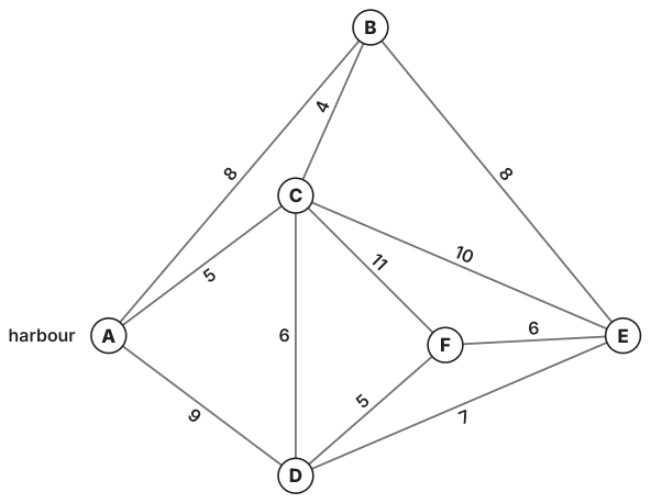
The island of Kerrin has six villages, A to F. The graph shows the roads between the villages, with the length of each road in kilometres. Village A has the harbour and the council's depot.
Original Photon diagram
The council plans to lay a fibre-optic cable alongside the roads so that every village is joined to the network.
(a) Use Kruskal's algorithm to find the minimum total length of cable needed. List the roads in the order in which you choose them.
[3]
Laying cable costs €38 000 per kilometre. A junction box costing €12 000 is also needed at every village where three or more lengths of cable meet.
(b) Find the total cost of the network in part (a).
[3]
(c) Explain why, in the network in part (a), damage to any single length of cable would cut off at least one village.
[1]
To protect against damage, an engineer suggests laying the cable as a ring: a cycle along the roads that passes through every village exactly once.
Let L km be the length of the shortest possible ring. The table shows some of the least distances, in kilometres, between the villages.
\begin{array}{|c|r|r|r|r|r|r|}\hline & A & B & C & D & E & F\\\hline A & \text{--} & 8 & 5 & 9 & \ldots & \ldots\\\hline B & 8 & \text{--} & 4 & 10 & 8 & \ldots\\\hline C & 5 & 4 & \text{--} & 6 & 10 & 11\\\hline D & 9 & 10 & 6 & \text{--} & 7 & 5\\\hline E & \ldots & 8 & 10 & 7 & \text{--} & 6\\\hline F & \ldots & \ldots & 11 & 5 & 6 & \text{--}\\\hline\end{array}
(d) (i) Complete the table.
[2]
(ii) Starting at A, apply the nearest neighbour algorithm to obtain an upper bound for L.
[2]
(iii) Delete vertex C to obtain a lower bound for L.
[3]
(iv) Hence write down an inequality satisfied by L.
[1]
(v) The ring found in part (d)(ii) uses only direct roads. Find how much more it costs than the network in part (a).
[2]
Each year an inspector drives along every road at least once, starting and finishing at the depot in A.
(e) (i) Explain why the inspector must drive along some roads more than once.
[1]
(ii) Find the length of the shortest inspection route, and state which roads are driven twice.
[4]
(iii) The council considers building a new road, of length x kilometres, directly between B and F. The new road would also need inspecting. Find the range of values of x for which the shortest inspection route would then be shorter than your answer to part (e)(ii).
[3]
(f) Suggest one way in which the cost model in part (b) could be improved.
[1]
Show solutionHide solution
(a) BC, AC, DF, CD, EF (AC and DF may swap), total 26 km.
(b) 26\times 38\,000=988\,000; one junction box at C; total €1 000 000.
(c) A tree has no cycles, so removing any edge leaves two parts with no path between them.
(d) (i) AE 15, AF 14, BF 14; (ii) A, C, B, E, F, D, A of length 37 km; (iii) 27+4+5=36 km; (iv) 36\le L\le 37; (v) 37\times 38\,000=1\,406\,000, which is €406 000 more.
(e) (i) A, B, C and F have odd degree; (ii) repeat BC and A-D-F, route length 79+18=97 km; (iii) 84+x<97, so 0<x<13.
(f) For example the cost per kilometre depends on the ground.

Final answer

(a) 26 km. (b) €1 000 000. (d) 36\le L\le 37; €406 000 more. (e) 97 km, repeating BC, AD, DF; 0<x<13.

Investigation

[27 marks]
Investigation 4: Aphids and ladybirds in a greenhouse.
Tomás grows peppers in a greenhouse. Aphids feed on the plants and ladybirds feed on the aphids. He models the two populations by
\frac{\mathrm{d}x}{\mathrm{d}t}=x(0.8-0.04y),\qquad \frac{\mathrm{d}y}{\mathrm{d}t}=y(0.01x-0.5),
where x is the number of aphids in hundreds, y is the number of ladybirds and t is the time in weeks.
(a) Find the two equilibrium points of the model, and interpret the non-zero equilibrium point in context.
[3]
At t=0 there are 4000 aphids and 15 ladybirds.
(b) Taking steps of 0.1 weeks, apply Euler's method to estimate how many aphids and how many ladybirds there are when t=0.2.
[4]
(c) Calculate \frac{\mathrm{d}y}{\mathrm{d}x} when t=0, and interpret its sign in context.
[2]
To study the populations close to the non-zero equilibrium, Tomás writes u=x-50 and v=y-20.
(d) Show that \frac{\mathrm{d}u}{\mathrm{d}t}=-2v-0.04uv, and find a similar expression for \frac{\mathrm{d}v}{\mathrm{d}t}.
[3]
When u and v are small, Tomás ignores the terms in uv and uses the linear system \frac{\mathrm{d}u}{\mathrm{d}t}=-2v, \frac{\mathrm{d}v}{\mathrm{d}t}=0.2u.
(e) (i) Find the eigenvalues of the matrix \begin{pmatrix}0&-2\\0.2&0\end{pmatrix}.
[2]
(ii) Hence describe the long-term behaviour of the two populations predicted by the linear system.
[1]
(iii) The solutions of the linear system have the form u=p\cos(\omega t)+q\sin(\omega t), where the eigenvalues are \pm\omega\mathrm{i}. Find the time taken for the populations to complete one cycle.
[2]
(f) Sketch the phase portrait of the linear system, showing the direction in which the trajectories are followed.
[2]
(g) (i) By separating the variables in \frac{\mathrm{d}v}{\mathrm{d}u}, show that every trajectory of the linear system satisfies 0.1u^2+v^2=c, where c is a constant.
[3]
(ii) Using the linear system and the starting values from part (b), find the largest and smallest numbers of aphids predicted.
[2]
Tomás sprays a pesticide that kills some insects of both species. His model becomes
\frac{\mathrm{d}x}{\mathrm{d}t}=x(0.6-0.04y),\qquad \frac{\mathrm{d}y}{\mathrm{d}t}=y(0.01x-0.6).
(h) Find the new non-zero equilibrium point, and comment on whether spraying helps Tomás in the long term.
[3]
Show solutionHide solution
(a) (0,0) and (50,20); 5000 aphids and 20 ladybirds can live together with both populations unchanged.
(b) After one step (40.8,\,14.85); after two steps x=41.6405, y=14.7134: about 4160 aphids and 14.7 ladybirds.
(c) -0.1875: \frac{\mathrm{d}x}{\mathrm{d}t}>0 and \frac{\mathrm{d}y}{\mathrm{d}t}<0, so aphids are rising while ladybirds are falling.
(d) \frac{\mathrm{d}u}{\mathrm{d}t}=(50+u)(-0.04v)=-2v-0.04uv and \frac{\mathrm{d}v}{\mathrm{d}t}=0.2u+0.01uv.
(e) (i) \lambda^2+0.4=0, so \lambda=\pm0.632\mathrm{i}; (ii) closed loops: both populations oscillate for ever; (iii) 2\pi/\sqrt{0.4}=9.93 weeks.
(f) Closed ellipses about the origin, followed anticlockwise.
(g) (i) -2v\,\mathrm{d}v=0.2u\,\mathrm{d}u, so -v^2=0.1u^2+K; (ii) c=35, u=\pm18.7, about 6870 and 3130 aphids.
(h) (60,15): spraying raises the aphid equilibrium from 5000 to 6000 and lowers the ladybirds from 20 to 15, so it makes the aphid problem worse.

Final answer

(a) (0,0), (50,20). (b) about 4160 aphids, 14.7 ladybirds. (c) -0.1875. (e) \pm0.632\mathrm{i}; 9.93 weeks. (g) c=35; 6870 and 3130 aphids. (h) (60,15).

From the book

Photon Guidebook: Mathematics Applications and Interpretation HL for the IB Diploma

Chapter 23 teaches paper 3: modelling investigations from the basics to full exam questions: how the IB asks it, every question type with a marked example, and these practice questions in three steps.

About the book