Statistics is a deceptively high-yield topic in IB Mathematics Analysis & Approaches HL. The formulas look gentle next to calculus, but the marks are routinely lost on small notational details — picking the wrong regression line, forgetting that adding a constant doesn't change the standard deviation, or multiplying 1.5 by the wrong quantity in the outlier fence. Examiners deliberately test these traps every session because they reveal whether a student really understands what each statistic measures, or is just feeding numbers into a GDC.
This cheatsheet condenses every formula, transformation rule, and exam-day decision from SL 4.1–4.4 and AHL 4.10–4.12 into one page you can revise from. It covers data classification, sampling, central tendency and dispersion, cumulative frequency and box plots, scatter diagrams and Pearson's $r$, the two regression lines, and the full attack plan for Paper 2 statistics questions. Scroll to the bottom for the printable PDF and the gated full library.
§1 — Data Types & Sampling SL 4.1
Data classifications
- Qualitative (categorical): described in words.
- Quantitative: always a number.
- Discrete: counted; takes specific values only.
- Continuous: measured; any value in a range.
- Population: entire group under study.
- Sample: representative subset of the population.
Five sampling methods
- Simple random (SRS) — random number generator; equal probability for every member.
- Systematic — every $k$-th member, where $k = N/n$.
- Stratified — random sample from each stratum.
- Quota — proportional to stratum size.
- Convenience — easiest accessible members.
Bias sources & reliability
| Bias source | Reliable data | Sufficient data |
|---|---|---|
| Sampling-frame exclusion | Repeatable results | Enough data points |
| Non-response | Similar findings | Supports conclusions |
| Poor question design | Controlled collection | Representative sample |
| Respondent dishonesty | Errors minimised | Errors logged |
§2 — Measures of Central Tendency SL 4.3
Mean
Grouped data: use the midpoint of each class as $x_i$. The result is an estimate — the exact mean is unknowable.
Median & mode
- Median (ordered data): if $n$ is odd, the $\dfrac{n+1}{2}$-th term; if $n$ is even, the mean of the $\dfrac{n}{2}$-th and $\left(\dfrac{n}{2}+1\right)$-th terms.
- Mode: the most frequent value.
- Modal class (grouped data): the class with the highest frequency.
§3 — Dispersion & Transformations SL 4.3
Key measures
GDC symbols: $\sigma_x$ is the population SD; $s_x$ is the sample SD. Use $\sigma_x$ unless told "sample standard deviation".
Transformation rules
| Transform | Effect on $\bar{x}$ | Effect on $\sigma$ |
|---|---|---|
| Add constant $k$ | $\bar{x} + k$ | unchanged |
| Subtract $k$ | $\bar{x} - k$ | unchanged |
| Multiply by $k$ | $k\bar{x}$ | $k\sigma$ |
| Divide by $k$ | $\bar{x}/k$ | $\sigma/k$ |
Variance follows the same rules but squared: adding $k$ leaves variance unchanged; multiplying by $k$ scales variance by $k^2$.
§4 — GDC TI-Nspire: Statistics SL 4.3, 4.4
1-Variable Statistics
- Path: Lists & Spreadsheet. Col A header =
data; Col B =freq. - Enter values and frequencies.
- Menu $\to$ 4 $\to$ 1 $\to$ 1 (1-Var Stats).
- X1 List =
data; Freq List =freq.
| $\bar{x}$ | mean |
| $\sigma_x$ | population SD |
| $s_x$ | sample SD |
| $n$ | count |
| $Q_1$, Med, $Q_3$ | quartiles |
| Min, Max | extremes |
Linear Regression ($y$ on $x$)
- Path: Lists & Spreadsheet. Col A =
xdata; Col B =ydata. - Menu $\to$ 4 $\to$ 1 $\to$ 3 (Lin Reg $mx + b$).
- X List =
xdata, Y List =ydata. Output: $m$, $b$, $r^2$, $r$, $\bar{x}$, $\bar{y}$. - For the $x$-on-$y$ line: swap the lists (old $y$ becomes X List), re-run regression. This gives $x = ay + b$.
- Scatter plot: Home $\to$ Data & Statistics $\to$ Menu $\to$ 4 $\to$ 6 $\to$ 1 (Show Linear).
§5 — Cumulative Frequency SL 4.2
Construction rules
- Plot cumulative frequency on the $y$-axis.
- Plot each cf value against the upper class boundary.
- Start at $(x_{\min},\, 0)$; end at $(x_{\max},\, n)$.
- Join with a smooth S-shaped curve (the ogive).
Reading off the curve
| Statistic | Read from $y$-axis at | Read $x$ |
|---|---|---|
| $Q_1$ | $n/4$ | $\to$ curve $\to$ down |
| Median $Q_2$ | $n/2$ | $\to$ curve $\to$ down |
| $Q_3$ | $3n/4$ | $\to$ curve $\to$ down |
| $p$-th percentile | $pn/100$ | $\to$ curve $\to$ down |
§6 — Box & Whisker Plots SL 4.2
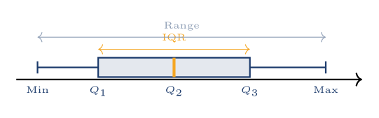
Five-number summary
Min — $Q_1$ — Median — $Q_3$ — Max. The IQR $= Q_3 - Q_1$ is the box width.
Outlier rule
A value $x$ is an outlier if:
- $x < Q_1 - 1.5 \cdot \text{IQR}$ (below the lower fence), or
- $x > Q_3 + 1.5 \cdot \text{IQR}$ (above the upper fence).
Outliers are plotted as $\times$. Whiskers extend to the last non-outlier.
What box plots show — and don't show
Shows: Min, $Q_1$, Median, $Q_3$, Max, IQR, outliers, skewness. Does NOT show: mean, $\sigma$, exact values, or the number of data points in each region (only the proportion — always 25% per quarter).
Skewness from a box plot
| Symmetric | Positive skew | Negative skew |
|---|---|---|
| Whiskers equal length; median centred in box | Right whisker longer; median closer to $Q_1$ | Left whisker longer; median closer to $Q_3$ |
| Data approx normal | Long tail to right | Long tail to left |
§7 — Scatter Plots & Pearson's $r$ SL 4.4
Describing a scatter diagram
Always describe three features:
- Direction: positive ($+$) / negative ($-$).
- Form: linear / non-linear (curved).
- Strength: strong / moderate / weak.
Independent variable ($x$) on the $x$-axis; dependent variable ($y$) on the $y$-axis.
Pearson's correlation coefficient $r$
$-1 \le r \le 1$ (use the GDC to compute).
| $r = +1$ | perfect positive |
| $|r| > 0.75$ | strong |
| $0.5 < |r| < 0.75$ | moderate |
| $|r| < 0.5$ | weak |
| $r = 0$ | no linear correlation |
| $r = -1$ | perfect negative |
Only valid for linear relationships! Always check the scatter plot before trusting $r$.
§8 — The Two Regression Lines SL 4.4, AHL 4.10
The two lines
- $y$-on-$x$ line: $y = ax + b$. Use when given $x$, predict $y$.
- $x$-on-$y$ line: $x = cy + d$. Use when given $y$, predict $x$.
Both lines pass through $(\bar{x},\, \bar{y})$ — solve simultaneously to recover $\bar{x}$ and $\bar{y}$.
Which line to use?
| Known | Want | Line |
|---|---|---|
| $x$ value | predict $y$ | $y$-on-$x$: $y = ax + b$ |
| $y$ value | predict $x$ | $x$-on-$y$: $x = cy + d$ |
To get the $x$-on-$y$ line on the GDC: swap the lists (old $y$ $\to$ X List, old $x$ $\to$ Y List), then re-run linear regression.
Interpreting regression coefficients in $y = ax + b$
| Gradient $a$ | Mean change in $y$ for each one-unit increase in $x$. Always state units. Must be contextualised: e.g. "population increases by 0.358 million per year". |
| Intercept $b$ | Predicted $y$ when $x = 0$. May have no physical meaning in context (e.g. negative price). Mention this if relevant. |
§9 — Interpolation, Extrapolation & Causation SL 4.4
| Interpolation | Extrapolation | Correlation $\neq$ Causation |
|---|---|---|
| Predict within data range | Predict outside data range | High $|r| \neq$ one causes other |
| More reliable | Less reliable / unreliable | Confounding variable may exist |
| Reliability $\propto |r|$ | Assume trend continues | Coincidence is possible |
| State if it is interp. | Must say "extrapolation" + "unreliable" | Never say "$x$ causes $y$" |
§10 — Exam Attack Plan All sections
When you see this in the question — reach for that:
| Question trigger | Reach for |
|---|---|
| "Describe the sampling method" | Name + defining feature (e.g. "systematic — every $k$-th") |
| "Identify a source of bias" | Name the type + give a specific example from context |
| "Sum $= S$, mean $= \mu$, find $n$" | $n = S/\mu$ directly |
| "Each value multiplied by $k$" | New mean $= k\bar{x}$, new $\sigma = k\sigma$, new variance $= k^2 \sigma^2$ |
| "Each value increased by $k$" | New mean $= \bar{x} + k$; $\sigma$ unchanged; variance unchanged |
| "Find the largest non-outlier" | $Q_3 + 1.5 \times \text{IQR}$ (upper fence); check if actual max $>$ fence |
| "Find minimum value of $Q_3$" | Set fence $=$ max, solve: $Q_3 + 1.5 \times \text{IQR} = \max$ |
| "Comment on reliability" | State interp./extrap. + "reliable/unreliable" + reason |
| "Estimate $y$ for given $x$" | Use the $y$-on-$x$ line |
| "Estimate $x$ for given $y$" | Use the $x$-on-$y$ line (swap lists on GDC) |
| "Find the mean of the data" | Both regression lines pass through $(\bar{x}, \bar{y})$ — solve simultaneously |
| "Interpret the value of $a$ in $y = ax + b$" | Change in $y$ per unit increase in $x$, with units, in context |
| "Describe the correlation" | Direction (positive/negative) + strength + linear |
| "Determine whether $X$ is an outlier" | Compute fence, compare $X$ to fence, state $X >$ or $<$ fence |
| "Compare two box plots" | Median, IQR, range, symmetry/skewness — address all four |
| "Modal class" | Class with highest frequency (grouped data only) |
| "Estimate the mean from grouped data" | Use midpoints; result is an estimate |
Top 5 marks lost — based on past papers
- Using the wrong regression line for prediction. If given $y$, use $x$-on-$y$. If given $x$, use $y$-on-$x$. Rearranging the wrong line costs all prediction marks.
- Outlier-fence formula error: writing $Q_3 + 1.5 \times Q_3$ instead of $Q_3 + 1.5 \times \text{IQR}$. Always compute IQR first, then multiply 1.5 by IQR — not by a quartile.
- Not saying "extrapolation" when asked about reliability. The exam expects the word explicitly. "The prediction may not be accurate" alone earns zero.
- Reading $s_x$ instead of $\sigma_x$ from GDC, or confusing variance and SD. Variance $= \sigma^2$. If the question asks for variance and you have $\sigma$, square it.
- Adding a constant and incorrectly changing the SD. "Each value increased by 5" changes only the mean. Standard deviation and variance are completely unaffected.
Worked Example — IB-Style Regression Analysis
Question (HL Paper 2 style — 8 marks)
For ten students at a Singapore IB school, the time $x$ (in hours) spent revising and the percentage score $y$ on the mock exam are recorded. The two regression lines obtained are $y = 4.2x + 28$ ($y$-on-$x$) and $x = 0.18y - 2.1$ ($x$-on-$y$). The data range is $4 \le x \le 18$.
(a) Find the mean revision time $\bar{x}$ and the mean score $\bar{y}$. (b) A student plans to revise for 12 hours. Estimate her score and comment on the reliability. (c) A student scored 95%. Estimate her revision time and comment.
Solution
- Both lines pass through $(\bar{x}, \bar{y})$. Substitute the second equation into the first: $y = 4.2(0.18y - 2.1) + 28$ (M1)
- Expand: $y = 0.756y - 8.82 + 28 \Rightarrow 0.244y = 19.18 \Rightarrow \bar{y} \approx 78.6$. Then $\bar{x} = 0.18(78.6) - 2.1 \approx 12.0$ (A1)(A1)
- (b) Given $x = 12$, use $y$-on-$x$: $\hat{y} = 4.2(12) + 28 = 78.4\%$ (M1)(A1)
- Reliability: $x = 12$ lies within the data range $[4, 18]$, so this is interpolation and the prediction is reasonably reliable. (R1)
- (c) Given $y = 95$, use $x$-on-$y$: $\hat{x} = 0.18(95) - 2.1 = 15.0$ hours (M1)(A1)
- Reliability: $y = 95$ is well outside the achieved range; substituting back, predicted $x = 15$ is still inside the range, but the score 95 is far from typical observed scores — borderline extrapolation. (R1)
Examiner's note: The trap in part (c) is using the $y$-on-$x$ line and rearranging $95 = 4.2x + 28$. That gives $x \approx 16.0$, which is wrong. You must use the $x$-on-$y$ line because $y$ is the known and $x$ is the prediction.
Common Student Questions
Which regression line should I use to predict $y$ from a known $x$?
How do I tell whether a value is an outlier in IB Math AA HL?
What is the difference between $\sigma_x$ and $s_x$ on the GDC?
If every data value is multiplied by $k$, how do the mean, SD and variance change?
When IB asks me to comment on the reliability of a prediction, what should I write?
Get the printable PDF version
Same cheatsheet, formatted for A4 print — keep it next to your study desk. Free for signed-in users.