Free worked solutions · 2026 Edition

IB Maths HL Paper 3 Chapter 6: Differential equations and their solution families worked solutions

Worked solutions to the investigations in Chapter 6 of Photon Guidebook: Mathematics HL Paper 3 for the IB Diploma (2026 Edition). Each solution shows every step with the mark it earns, the way an IB mark scheme does.

Chapter 6 of 18
7 practice questions
2 Going further
Free, no sign-up

Start with Investigations All 18 chapters

Investigations

The practice investigations of the chapter, each with its full worked solution and mark scheme.

Investigation 1

[18 marks]

This question asks you to model the amount of salt in a tank as salt water flows in and out.

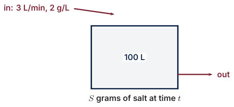
A tank holds 100 litres of pure water. From t=0, salt water with 2 grams of salt per litre flows in at 3 litres per minute, and the well-mixed liquid flows out at the same rate. Let S grams be the mass of salt in the tank at time t minutes.

(a) Show that \dfrac{dS}{dt}=6-0.03S.

[2]

(b) Solve the equation to find S in terms of t.

[4]

(c) Find the time at which the tank contains 100 g of salt.

[2]

(d) State the long-term mass of salt and explain it in context.

[2]

The outflow is now reduced to 2 litres per minute while the inflow is unchanged, so the volume increases. Again the tank starts with 100 litres of pure water.

(e) Show that \dfrac{dS}{dt}=6-\dfrac{2S}{100+t}.

[2]

(f) Solve this equation with an integrating factor, and find the concentration of salt after 50 minutes.

[6]

Show solutionHide solution

(a) Salt enters at 2\times3=6 g per minute (A1). The volume stays 100 L, so the concentration is \frac S{100} and salt leaves at 3\times\frac S{100}=0.03S g per minute (A1). Hence \frac{dS}{dt}=6-0.03S.

(b) \displaystyle\int\frac{dS}{6-0.03S}=\int dt (M1) gives -\frac1{0.03}\ln|6-0.03S|=t+c (A1). With S=0 at t=0, c=-\frac1{0.03}\ln6 (M1). Then 6-0.03S=6e^{-0.03t}, so S=200\left(1-e^{-0.03t}\right) (A1).

(c) 100=200\left(1-e^{-0.03t}\right) gives e^{-0.03t}=\frac12 (M1), so t=\frac{\ln2}{0.03}=23.1 minutes (A1).

(d) As t\to\infty, S\to200 g (A1). This is 2 g per litre \times 100 L: the tank ends with the concentration of the incoming water (R1).

(e) The volume is 100+3t-2t=100+t litres (A1). The concentration is \frac S{100+t}, so salt leaves at 2\times\frac S{100+t} g per minute, and with the inflow 6 the equation follows (A1).

(f) Standard form \frac{dS}{dt}+\frac{2}{100+t}S=6, and \int\frac2{100+t}dt=2\ln(100+t) (M1). The integrating factor is (100+t)^2 (A1). Then \frac d{dt}\left[S(100+t)^2\right]=6(100+t)^2 (M1), so S(100+t)^2=2(100+t)^3+C (A1). With S(0)=0, C=-2\times10^6, and S=2(100+t)-\frac{2\times10^6}{(100+t)^2} (A1). At t=50, S=300-88.9=211.1 g, and the concentration is \frac{211.1}{150}=1.41 g per litre (A1).

Final answer

Salt in a tank. (b) S=200\left(1-e^{-0.03t}\right). (c) 23.1 minutes. (d) 200 g. (f) S=2(100+t)-\dfrac{2\times10^6}{(100+t)^2}; 211.1 g, 1.41 g per litre.

Investigation 2

[18 marks]

This question asks you to read a slope field, solve the equation it comes from and describe its solution curves.

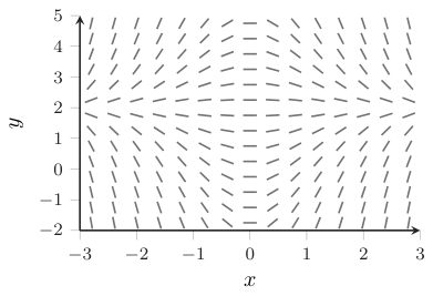
The slope field of \dfrac{dy}{dx}=x(2-y) is shown in the figure.

(a) Find the gradient of a solution curve at (2,0) and at (-2,0).

[2]

(b) Show that y=2 is a solution, and explain from the equation why, for x>0, the segments above this line slope down and those below it slope up.

[3]

(c) Find the equation of the curve along which every solution has gradient 1.

[2]

(d) Find the solution whose graph passes through the point (0,-1).

[5]

(e) For this solution, write down the coordinates of the minimum point and the equation of the horizontal asymptote.

[2]

(f) Show that the graph of this solution has points of inflexion at x=\pm1, and find their y-coordinate.

[4]

Show solutionHide solution

(a) At (2,0): 2(2-0)=4 (A1). At (-2,0): -2(2-0)=-4 (A1).

(b) If y=2 then \frac{dy}{dx}=0 and x(2-2)=0, so the equation holds (A1). For x>0 and y>2, 2-y<0 so the gradient is negative (R1). For x>0 and y<2, 2-y>0 so the gradient is positive (R1). Both point towards the line.

(c) x(2-y)=1 (M1), so y=2-\frac1x (A1).

(d) \displaystyle\int\frac{dy}{2-y}=\int x\,dx (M1) gives -\ln|2-y|=\frac{x^2}2+c (A1). Then |2-y|=Be^{-x^2/2} (M1), so y=2+Ae^{-x^2/2} (A1). With y=-1 at x=0, A=-3, and y=2-3e^{-x^2/2} (A1).

(e) \frac{dy}{dx}=3xe^{-x^2/2} changes sign from negative to positive at x=0, so the minimum point is (0,-1) (A1). As x\to\pm\infty, y\to2, so the asymptote is y=2 (A1).

(f) \frac{d^2y}{dx^2}=3e^{-x^2/2}-3x^2e^{-x^2/2}=3(1-x^2)e^{-x^2/2} (M1 A1). This is zero at x=\pm1 and changes sign there (R1). The y-coordinate is 2-3e^{-1/2}=0.180 (A1).

Final answer

A field with a flat line. (a) 4, −4. (c) y=2-\dfrac1x. (d) y=2-3e^{-x^2/2}. (e) (0,-1); y=2. (f) x=\pm1, y=2-3e^{-1/2}=0.180.

Investigation 3

[20 marks]

This question asks you to model the depth of water in a tub that drains through a small hole, and to find where Euler's method breaks down.

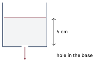
Water drains from a cylindrical tub through a hole in its base. The depth of the water is h centimetres at time t seconds, and \dfrac{dh}{dt}=-0.2\sqrt h. At t=0 the depth is 25 cm.

(a) Solve the differential equation to show that h=(5-0.1t)^2.

[4]

(b) Find the time at which the tub is empty.

[2]

(c) Find the time at which the depth has fallen to half of its original value.

[3]

(d) Find \dfrac{dh}{dt} when h=4, and explain why the water drains more slowly as the depth falls.

[2]

(e) Use Euler's method with a step of 10 seconds to estimate h at t=10, 20 and 30.

[4]

(f) Find the percentage error in each estimate, and show that the next Euler step cannot be taken.

[3]

(g) Explain why the formula h=(5-0.1t)^2 cannot describe the depth for t>50.

[2]

Show solutionHide solution

(a) \displaystyle\int h^{-1/2}\,dh=\int-0.2\,dt (M1) gives 2\sqrt h=-0.2t+c (A1). With h=25 at t=0, c=10 (M1), so \sqrt h=5-0.1t (A1) and h=(5-0.1t)^2.

(b) h=0 when 5-0.1t=0 (M1), that is at t=50 seconds (A1).

(c) (5-0.1t)^2=12.5 (M1). Taking the positive root, 5-0.1t=\sqrt{12.5} (A1), so t=10\left(5-\sqrt{12.5}\right)=14.6 seconds (A1).

(d) \frac{dh}{dt}=-0.2\times2=-0.4 cm per second (A1). The rate is proportional to \sqrt h, so it shrinks as h shrinks (R1).

(e) h_{n+1}=h_n-10\left(0.2\sqrt{h_n}\right) (M1). h(10)=25-2\times5=15 (A1). h(20)=15-2\sqrt{15}=7.254 (A1). h(30)=7.254-2\sqrt{7.254}=1.867 (A1).

(f) Exact values are 16, 9, 4 (M1). The errors are \frac{16-15}{16}=6.25\%, \frac{9-7.254}{9}=19.4\% and \frac{4-1.867}{4}=53.3\% (A1). The next step would give 1.867-2\sqrt{1.867}=-0.866, a negative depth, and then \sqrt h is not defined (R1).

(g) For t>50 the formula (5-0.1t)^2 increases again, but water cannot flow back in (A1). Also \sqrt h=5-0.1t would be negative, which is impossible (R1).

Final answer

A tub with a hole in it. (a) proof. (b) 50 s. (c) 14.6 s. (d) −0.4 cm per second. (e) 15, 7.254, 1.867. (f) 6.25%, 19.4%, 53.3%; the next depth is negative. (g) the formula rises again.

Investigation 4

[20 marks]

This question asks you to measure the error of Euler's method on an equation you can also solve exactly.

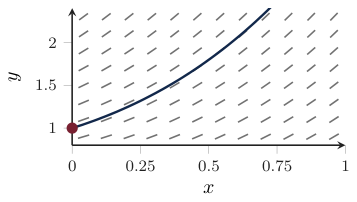
Consider \dfrac{dy}{dx}=x+y, with y=1 when x=0. The slope field and the solution curve are shown in the figure.

(a) Taking steps of 0.1, apply Euler's method to estimate y at x=0.5.

[4]

(b) Use an integrating factor to solve the equation exactly, and find the exact value of y when x=0.5.

[5]

(c) Repeat (a) with h=0.05.

[3]

(d) Find the error in each estimate and the ratio of the two errors.

[3]

(e) Suggest the error when h=0.025, and the step needed for an error below 0.001.

[3]

(f) Explain, using the shape of the solution curve, why Euler's method underestimates y here.

[2]

Show solutionHide solution

(a) y_{n+1}=y_n+0.1(x_n+y_n) (M1). y(0.1)=1.1 and y(0.2)=1.1+0.1(0.1+1.1)=1.22 (A1). y(0.3)=1.362 and y(0.4)=1.5282 (A1). y(0.5)=1.5282+0.1(0.4+1.5282)=1.72102 (A1).

(b) \frac{dy}{dx}-y=x, so the integrating factor is e^{-x} (M1 A1). Then \frac d{dx}\left(ye^{-x}\right)=xe^{-x} (M1) and by parts ye^{-x}=-xe^{-x}-e^{-x}+C (A1). With y(0)=1, C=2, so y=2e^x-x-1 and y(0.5)=2e^{0.5}-1.5=1.79744 (A1).

(c) Ten steps of 0.05 with y_{n+1}=y_n+0.05(x_n+y_n) (M1): y(0.05)=1.05, y(0.1)=1.105 (A1). Continuing, y(0.5)=1.75779 (A1).

(d) Errors: 1.79744-1.72102=0.0764 (A1) and 1.79744-1.75779=0.0397 (A1). The ratio is \frac{0.0764}{0.0397}=1.93 (A1).

(e) The error is about halved when h is halved, so the ratio is close to 2 (M1). For h=0.025 the error is about 0.020 (A1). The error is about 0.793h, so an error below 0.001 needs h<0.0013 (A1). A check on the GDC: h=0.00125 gives 0.00103, which is still too big, and h=0.001 gives 0.000824.

(f) \frac{d^2y}{dx^2}=2e^x>0, so the solution curve is concave up (A1). Each Euler step follows a tangent, and a tangent to a concave-up curve lies below it, so every step falls short and the shortfalls add up (R1).

Final answer

How good is Euler's method. (a) 1.72102. (b) y=2e^x-x-1, y(0.5)=1.79744. (c) 1.75779. (d) 0.0764, 0.0397, ratio 1.93. (e) about 0.020; h near 0.001. (f) the curve is concave up.

Investigation 5

[22 marks]

This question asks you to solve a homogeneous differential equation using partial fractions, and to use the way its solution curves scale.

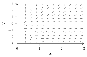
Consider \dfrac{dy}{dx}=\dfrac{y^2+2xy}{x^2} for x>0. The slope field is shown in the figure.

(a) Writing y=vx, show that x\dfrac{dv}{dx}=v(v+1).

[3]

(b) Hence show that the general solution can be written as \dfrac y{x+y}=Ax, where A is a constant.

[6]

(c) Find the solution with y=1 when x=1, giving y in terms of x.

[3]

(d) State the interval of x on which this solution is defined, and describe what happens to y as x approaches the upper end of the interval.

[3]

(e) Show that, if y=f(x) is a solution, then so is y=kf\left(\dfrac xk\right) for every k>0.

[4]

(f) Find the values of v for which the gradient of a solution curve is 3, and describe the lines on which this happens.

[3]

Show solutionHide solution

(a) \frac{dy}{dx}=v+x\frac{dv}{dx} (M1). The right-hand side is \frac{v^2x^2+2vx^2}{x^2} (M1) =v^2+2v (A1). Hence x\frac{dv}{dx}=v^2+2v-v=v(v+1).

(b) \displaystyle\int\frac{dv}{v(v+1)}=\int\frac{dx}x (M1). Partial fractions: \frac1{v(v+1)}=\frac1v-\frac1{v+1} (M1). So \ln|v|-\ln|v+1|=\ln x+c (A1 A1). Then \frac v{v+1}=Ax (M1). Since \frac v{v+1}=\frac{y/x}{(y+x)/x}=\frac y{x+y} (A1), the result follows.

(c) At (1,1): \frac12=A (M1 A1). Then 2y=x(x+y), so y(2-x)=x^2 and y=\frac{x^2}{2-x} (A1).

(d) The solution is defined for 0<x<2 (A1). As x\to2^- the numerator tends to 4 and the denominator to 0^+ (M1), so y\to+\infty (A1).

(e) Let g(x)=kf\left(\frac xk\right). Then g'(x)=f'\left(\frac xk\right) (M1 A1). Since f is a solution, f'(u)=\frac{f(u)^2+2uf(u)}{u^2} with u=\frac xk (A1). Now f(u)=\frac gk, so f'(u)=\frac{g^2/k^2+2xg/k^2}{x^2/k^2}=\frac{g^2+2xg}{x^2} (R1), which is the equation for g.

(f) The gradient on y=vx is v^2+2v (M1). Solving v^2+2v=3 gives v=1 or v=-3 (A1). The gradient is 3 along the rays y=x and y=-3x (A1).

Final answer

Curves that scale. (c) y=\dfrac{x^2}{2-x}. (d) 0<x<2; y\to\infty. (f) v=1 or −3: the rays y=x and y=-3x.

Investigation 6

[25 marks]

This question asks you to solve a first-order linear equation and to find where the stationary points of its solution curves lie.

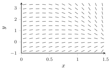
Consider \dfrac{dy}{dx}+y\tan x=\cos x for 0\le x<\dfrac\pi2. The slope field is shown in the figure.

(a) Show that \sec x is an integrating factor.

[3]

(b) Hence show that the general solution is y=(x+C)\cos x.

[3]

(c) Find the solution with y=2 when x=0, and find the coordinates of its maximum point.

[4]

(d) Show that every stationary point of every solution curve lies on the curve y=\dfrac{\cos^2x}{\sin x}.

[3]

(e) Show that the solution with constant C has exactly one stationary point for 0<x<\dfrac\pi2 when C>-\dfrac\pi2, and none otherwise.

[6]

(f) Describe how the stationary point moves along the curve in (d) as C increases.

[3]

(g) Show that the curve y=(x+C)\cos x passes through \left(\dfrac\pi2,0\right) for every value of C, and find its gradient there in terms of C.

[3]

Show solutionHide solution

(a) The integrating factor is e^{\int\tan x\,dx} (M1). \int\tan x\,dx=-\ln\cos x=\ln\sec x (A1) for 0\le x<\frac\pi2, where \cos x>0. So the factor is e^{\ln\sec x}=\sec x (A1).

(b) Multiplying by \sec x, \frac d{dx}\left(y\sec x\right)=\sec x\cos x=1 (M1 A1). Integrating, y\sec x=x+C (A1), so y=(x+C)\cos x.

(c) y(0)=C=2, so y=(x+2)\cos x (A1). At a stationary point \cos x-(x+2)\sin x=0 (M1). The GDC gives x=0.395 (A1) and y=2.21 (A1).

(d) At a stationary point \frac{dy}{dx}=0, so the equation gives y\tan x=\cos x (M1 A1). Then y=\frac{\cos x}{\tan x}=\frac{\cos^2x}{\sin x} (A1).

(e) \frac{dy}{dx}=\cos x-(x+C)\sin x=0 (M1), and since \sin x\ne0 for 0<x<\frac\pi2 this is C=\cot x-x=g(x) (A1). g'(x)=-\operatorname{cosec}^2x-1<0 (M1 A1), so g is strictly decreasing and takes each value at most once (R1). As x\to0^+, g\to\infty, and g\left(\frac\pi2\right)=-\frac\pi2. By continuity g takes every value in \left(-\frac\pi2,\infty\right) exactly once, so there is exactly one stationary point if C>-\frac\pi2 and none otherwise (R1).

(f) g is decreasing, so a larger C means a smaller x (A1). The stationary point therefore moves towards the y-axis, and x\to0 as C\to\infty (A1). On the curve y=\frac{\cos^2x}{\sin x}, y\to\infty as x\to0^+, so the point also moves up the curve without bound (A1).

(g) y\left(\frac\pi2\right)=\left(\frac\pi2+C\right)\cos\frac\pi2=0 (A1). \frac{dy}{dx}=\cos x-(x+C)\sin x (M1), and at x=\frac\pi2 this is -\left(\frac\pi2+C\right) (A1).

Final answer

Where the stationary points lie. (c) y=(x+2)\cos x, maximum at (0.395,\,2.21). (e) C=\cot x-x is strictly decreasing from \infty to -\frac\pi2. (f) towards the y-axis and up the curve. (g) gradient -\left(\frac\pi2+C\right).

Investigation 7

[25 marks]

This question asks you to solve a non-linear differential equation by a substitution and to study its solutions.

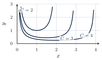
Consider \dfrac{dy}{dx}+\dfrac yx=xy^2 for x>0. Some members of the family of solutions found in part (b) are shown in the figure.

(a) Show that the substitution u=\dfrac1y transforms the equation into \dfrac{du}{dx}-\dfrac ux=-x.

[4]

(b) Solve this linear equation, and hence show that y=\dfrac1{Cx-x^2}.

[6]

(c) Find the solution with y=\dfrac12 when x=1.

[2]

(d) For this solution, write down where its graph has vertical asymptotes, and the interval of x, containing x=1, on which the solution is defined.

[3]

(e) Find the minimum value of y on this interval.

[3]

(f) Show that for every C>0 the solution has a minimum point, and find the curve on which all the minimum points lie.

[5]

(g) Describe the solutions with C\le0.

[2]

Show solutionHide solution

(a) Divide the equation by y^2: \frac1{y^2}\frac{dy}{dx}+\frac1{xy}=x (M1). With u=\frac1y, \frac{du}{dx}=-\frac1{y^2}\frac{dy}{dx} (A1). Substituting gives -\frac{du}{dx}+\frac ux=x (M1 A1), which rearranges to \frac{du}{dx}-\frac ux=-x.

(b) The integrating factor is e^{\int-\frac1x\,dx} (M1) =\frac1x (A1). Then \frac1x\frac{du}{dx}-\frac u{x^2}=-1, that is \frac d{dx}\left(\frac ux\right)=-1 (M1 A1). Integrating, \frac ux=-x+C (M1 A1), so u=Cx-x^2 and y=\frac1u=\frac1{Cx-x^2}.

(c) \frac1{C-1}=\frac12 gives C=3 (M1), so y=\frac1{3x-x^2} (A1).

(d) 3x-x^2=x(3-x)=0 at x=0 and x=3, the vertical asymptotes (A1 A1). The solution is defined for 0<x<3 (A1).

(e) y is least where 3x-x^2 is greatest (M1). The greatest value of 3x-x^2 is \frac94 at x=\frac32 (A1), so the minimum value of y is \frac49 (A1).

(f) For C>0 the denominator Cx-x^2 is positive on 0<x<C and has its greatest value at x=\frac C2 (M1 A1). So y has a minimum point at x=\frac C2 with y=\frac4{C^2} (A1). Eliminating C: C=2x, so y=\frac4{4x^2} (M1), which gives y=\frac1{x^2} (A1).

(g) For C\le0 and x>0 the denominator Cx-x^2 is negative, so y<0 and the solution is defined for all x>0 (A1). It tends to 0 from below as x\to\infty and to -\infty as x\to0^+ (A1).

Final answer

A substitution that makes it linear. (b) \left(\dfrac ux\right)'=-1. (c) y=\dfrac1{3x-x^2}. (d) x=0, x=3; 0<x<3. (e) \dfrac49 at x=\dfrac32. (f) minimum at x=\dfrac C2, y=\dfrac4{C^2}; locus y=\dfrac1{x^2}. (g) y<0 for all x>0, y\to0^- as x\to\infty.

Going further

Beyond the syllabus: the worked examples and investigations of the chapter's Going further pages.

Investigation

[28 marks]

Worked investigation 1: A drink in a warming room.

This question asks you to model the temperature of a drink in a room whose temperature is rising.

At 08:00 a cup of coffee at 90^\circC is placed in a kitchen. The kitchen temperature, in ^\circC, is 20+0.5t, where t is the number of minutes since 08:00. The temperature of the coffee, T\,{}^\circC, satisfies \dfrac{dT}{dt}=-0.1\left(T-(20+0.5t)\right).

(a) Explain what the constant 0.1 and the expression T-(20+0.5t) represent.

[2]

(b) Show that the equation can be written as \dfrac{dT}{dt}+0.1T=2+0.05t, and find an integrating factor.

[3]

(c) Find the general solution.

[5]

(d) Find the particular solution with T=90 when t=0.

[2]

(e) Find the time at which the coffee is coolest, and its temperature then.

[4]

(f) Show that, after a long time, the coffee is always about 5^\circC cooler than the kitchen, and explain why.

[3]

(g) Use Euler's method with a step of 1 minute to estimate T when t=2, and find the percentage error.

[4]

(h) Give one reason why the model may not be valid two hours after 08:00.

[2]

(i) For a kitchen temperature a+bt and cooling constant k, find how far below the kitchen temperature the coffee settles.

[3]

Show solutionHide solution

(a) T-(20+0.5t) is how many ^\circC the coffee is above the kitchen at time t (A1); 0.1 per minute is the fraction of that excess lost each minute; the minus sign makes a hot coffee cool (A1).

(b) \dfrac{dT}{dt}=-0.1T+0.1(20+0.5t)=-0.1T+2+0.05t (M1); \dfrac{dT}{dt}+0.1T=2+0.05t (AG); \displaystyle\int0.1\,dt=0.1t (M1); integrating factor e^{0.1t} (A1).

(c) \dfrac{d}{dt}\left(e^{0.1t}T\right)=(2+0.05t)e^{0.1t} (M1); \displaystyle\int(2+0.05t)e^{0.1t}\,dt=10(2+0.05t)e^{0.1t}-\int0.5\,e^{0.1t}\,dt (M1); =(20+0.5t)e^{0.1t}-5e^{0.1t}=(15+0.5t)e^{0.1t} (A1); e^{0.1t}\,T=(15+0.5t)e^{0.1t}+C (A1); T=15+0.5t+Ce^{-0.1t} (A1).

(d) 90=15+0+C (M1); C=75, so T=15+0.5t+75e^{-0.1t} (A1).

(e) \dfrac{dT}{dt}=0.5-7.5\,e^{-0.1t} (M1); 0.5-7.5\,e^{-0.1t}=0, so e^{-0.1t}=\dfrac1{15} (A1); t=10\ln15=27.1 minutes (A1); T=15+5\ln15+75\times\dfrac1{15}=20+5\ln15=33.5\,{}^\circC (A1).

(f) T-(20+0.5t)=-5+75e^{-0.1t} (M1); As t\to\infty, e^{-0.1t}\to0, so the difference tends to -5: the coffee is about 5^\circC below the kitchen (A1); To warm at the kitchen rate 0.5 the coffee needs -0.1\times(\text{difference})=0.5, that is a difference of -5 (R1).

(g) T_{n+1}=T_n+h\left[-0.1\left(T_n-(20+0.5t_n)\right)\right] with h=1 (M1); T(1)=90-0.1(90-20)=83 (A1); T(2)=83-0.1(83-20.5)=76.75 (A1); Exact T(2)=16+75e^{-0.2}=77.405, so the error is \dfrac{77.405-76.75}{77.405}=0.846\% (A1).

(h) The formula gives a kitchen at 20+0.5\times120=80^\circC at 10:00 (A1); A room cannot keep warming at a constant rate for ever, so the model fails after some time (R1).

(i) Try T=p+qt in \dfrac{dT}{dt}+kT=k(a+bt): q+k(p+qt)=ka+kbt (M1); Compare the t terms: q=b. Compare constants: b+kp=ka, so p=a-\dfrac bk (A1); The term Ce^{-kt} dies away, so T\to a-\dfrac bk+bt, which is \dfrac bk below a+bt (A1).

Final answer

(b) e^{0.1t}. (c) T=15+0.5t+Ce^{-0.1t}. (d) C=75. (e) t=10\ln15=27.1 min, T=20+5\ln15=33.5\,{}^\circC. (g) 83, 76.75; error 0.846\%. (i) \dfrac bk.

Investigation

[24 marks]

Worked investigation 2: A family of hyperbolas from a homogeneous equation.

This question asks you to solve a homogeneous differential equation and to describe its family of solution curves.

Consider \dfrac{dy}{dx}=\dfrac{x^2+y^2}{2xy} for x>0, y>0.

(a) Find the gradient of the solution curve through the point (1,2).

[1]

(b) Writing y=vx, where v is a function of x, show that x\dfrac{dv}{dx}=\dfrac{1-v^2}{2v}.

[4]

(c) Hence show that the general solution is x^2-y^2=Ax, where A is a constant.

[5]

(d) Find the solution curve through (2,1), and state the values of x for which it is defined.

[3]

(e) Show that this curve approaches the line y=x-\dfrac34 as x\to\infty.

[3]

(f) Show that the line y=x is itself a solution curve.

[2]

(g) Show that the gradient of every solution curve is at least 1, and explain where it equals 1.

[3]

(h) Describe how the solution curves with A>0 differ from those with A<0.

[3]

Show solutionHide solution

(a) \dfrac{dy}{dx}=\dfrac{1^2+2^2}{2(1)(2)}=\dfrac54 (A1).

(b) \dfrac{dy}{dx}=\dfrac{d}{dx}(vx) (M1); =v+x\dfrac{dv}{dx} (A1); v+x\dfrac{dv}{dx}=\dfrac{x^2+v^2x^2}{2x\cdot vx} (M1); =\dfrac{1+v^2}{2v} (A1); x\dfrac{dv}{dx}=\dfrac{1+v^2}{2v}-v=\dfrac{1-v^2}{2v} (AG).

(c) \dfrac{2v}{1-v^2}\,dv=\dfrac1x\,dx (M1); -\ln|1-v^2|=\ln x+c (A1 A1); |1-v^2|=\dfrac{e^{-c}}{x}, so 1-v^2=\dfrac Ax (M1); 1-\dfrac{y^2}{x^2}=\dfrac Ax (A1); x^2-y^2=Ax (AG).

(d) 2^2-1^2=A\cdot2 (M1); A=\dfrac32 (A1); y=\sqrt{x^2-\tfrac32x}, defined for x>\tfrac32 (A1).

(e) \sqrt{x^2-\tfrac32x}-\left(x-\tfrac34\right)=\dfrac{\left(x^2-\frac32x\right)-\left(x-\frac34\right)^2}{\sqrt{x^2-\frac32x}+x-\frac34} (M1); =\dfrac{-\frac9{16}}{\sqrt{x^2-\frac32x}+x-\frac34} (A1); The denominator \to\infty, so the difference \to0 from below (R1).

(f) On y=x: \dfrac{dy}{dx}=1 and \dfrac{x^2+x^2}{2x\cdot x}=1 (M1); The two sides agree for every x>0, so y=x is a solution curve (A1).

(g) \dfrac{x^2+y^2}{2xy}-1=\dfrac{x^2+y^2-2xy}{2xy} (M1); =\dfrac{(x-y)^2}{2xy} (A1); x,y>0, so this is \ge0, and it is 0 only when y=x: the gradient is 1 only on the line y=x (R1).

(h) A>0: x^2-y^2=Ax>0, so y<x. The curve y=\sqrt{x^2-Ax} starts on the x-axis at (A,0) and exists for x\ge A (A1); A<0: y^2=x^2+|A|x>x^2, so y>x. The curve starts at the origin and exists for all x>0 (A1); Both kinds approach the line y=x-\dfrac A2, parallel to y=x (A1).

Final answer

(a) \frac54. (d) y=\sqrt{x^2-\frac32x}, x>\frac32. (e) the difference tends to 0 from below. (g) gradient -1=\frac{(x-y)^2}{2xy}\ge0. (h) A>0 below y=x; A<0 above; asymptote y=x-\frac A2.

From the book

Photon Guidebook: Mathematics HL Paper 3 for the IB Diploma

Chapter 6 teaches differential equations and their solution families: how the IB builds this kind of Paper 3 question, the techniques, marked worked investigations, and practice investigations like these.

About the book